Deep learning based curb detection with Lidar①

WANG Xiaohua (王小华), LIAO Zhonghe, MA Pin, MIAO Zhonghua

(School of Mechatronic Engineering and Automation, Shanghai University, Shanghai 200444, P.R.China)

Abstract Curb detection provides road boundary information and is important to road detection. However, curb detection is challenging due to the problems such as various curb shapes, colour, discontinuity. In this work, a novel learning-based method for curb detection is proposed using Lidar point clouds, considering that Lidars are not sensitive to illumination and are relatively stable to weather conditions. A deep neural network, named EdgeNet, is constructed and trained, which handles point clouds in an end-to-end way. After EdgeNet is properly trained, curb points are then segmented in the neural network output. In order to train,a curb point annotation algorithm is also designed to generate training dataset. The curb detection method works well with different road scenarios including intersections. The experimental results validate the effectiveness and robustness of this curb detection method.

Key words: curb detection, EdgeNet, curb annotation algorithm

0 Introduction

Detecting road boundary is necessary for vehicles with full or partial autonomy. Without road boundary information, it would be difficult for vehicles to understand their surroundings and to generate behaviour plans. Curb detection is developing rapidly. Many curb detection methods have been proposed.

Methods[1-2]of model curbs use parabolic curves and random sample consensus[3](RANSAC) algorithm to remove points that do not match the parabolic model. Ref.[1] employed three spatial cues to detect candidate curb points, i. e., elevation difference, gradient value, and normal orientation. A particle filter was also used to track curbs. Ref.[2] detected curb points by using integral laser points (ILP) features. In both methods, parameters are preset and manual adjustment is required.

Ref.[4] used a Gaussian differential filter to process single line Lidar data. The method is simple and fast, which is implemented in Defense Advanced Research Projects Agency (DARPA) urban challenge vehicles. Kalman filters[5]are also used to detect curbs. Ref.[6] proposed curb detection and tracking method, based on an extended Kalman filter using 2D Lidar data. Other methods[7-9]use the probabilistic interacting multiple model (IMM) algorithm, which contains a finite number of Kalman filters, to determine the curb existence. Filter-based methods also require pre-selected thresholds and filter parameters.

Considering that curbs are not always continuous,Ref.[10] proposed a sliding-beam model[11]to segment the road with intersections using Lidar data. This method uses a series of beams emitted from selected launching point, where beams are evenly spaced with a given angular resolution. The sliding-beam model is able to segment the current road and the road ahead by moving the launching point. A probabilistic beam model based on 3D point cloud[12]is proposed to segment the intersections. A machine learning method[13-14]is used to classify road shapes using beam models.

Cameras and ultrasonic sensors are also used for curb detection. Ref.[15] used an on-board camera to detect curbs. Ref.[16] used multiple ultrasonic sensors to implement a low-cost curb detection system. In general, vision-based method would suffer from insufficient illumination and bad weather condition, while radar-based method has comparatively lower resolution.

In recent years, deep learning has been applied to point cloud segmentation and classification, which brings new ideas for curb detection. One way of point cloud deep learning is to project a 3D point cloud onto a 2D plane, and then process the plane as a 2D image, for example, MV3D[17]and AVOD[18]. Curbs are detected by deep learning on a 2D bird-eye’s view of 3D Lidar point clouds[19-20].

In 2017, Refs[21,22] started the pioneering work of PointNet and PointNet ++, which provide an endto-end way to classify and segment point clouds. A PointNet++ grasping approach[23]is proposed, which can directly predict the poses, categories, and scores(qualities) of all the grasps. Dynamic graph convolutional neural network[24](DGCNN) is proposed, which learns to semantically group points by dynamically updating a graphic relation from layer to layer.

In this work, an end-to-end neural network (EdgeNet) is proposed for curb detection, which avoids manual parameter adjustments and provides good segmentation of curb points and non-curb points. The rest of the paper is organized as follows. Section 1 introduces training dataset preparation and the EdgeNet structure. Section 2 performs contrast experiments using PointNet, DGCNN and EdgeNet. Section 3 draws the conclusions.

1 Materials and methods

Since no open-source point cloud dataset with curb labels is available, a curb annotation algorithm is designed to annotate curb points for training EdgeNet.In this dataset, data are obtained from the roads on Baoshan campus of Shanghai University. The details of the algorithm are illustrated in subsection 1.1 -1.3.The structure of EdgeNet is then introduced in subsection 1.4.

1.1 Curb annotation algorithm

Fig.1 shows that how Lidar lines intersect a curb.Note that, when a Lidar line scans across a curb, the distance from Lidar center to the curb is shorter compared with that to the ground, i.e., the point distance L2(on the curb) is shorter than L1(on the ground) on one scan line, as shown in Fig.1(b) and Fig.1(c).In Fig.1(b) and Fig.1(c),‘a’ and ‘b’ are the two intersecting end points. L1 and L2 denote the distance from ‘a’ and ‘b’ to the coordinate origin, respectively. The coordinate origin is the Lidar center (xdirection points to the front;yandzaxis are set up according to the right-hand rule).

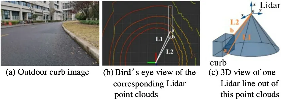
Fig.1 Diagrams of Lidar lines intersect a curb

According to the analysis above, a curb annotation algorithm is designed based on the distance difference of point clouds. This algorithm detects the curb points by looking for curb endpoints.

Fig.2 shows the flowchart of the curb annotation algorithm. The algorithm considers Lidar lines one by one. First of all, cloud points of one Lidar line is projected ontoXOYplane. For each point on the Lidar line, the distance to the origin is calculated as shown in Eq.(1). More important, distance variance of each point is calculated as shown in Eq.(2). The maximum and minimum of the distance variance are then selected as two curb endpoints, where the points in between are marked as curb points and the rest ones are non-curb points.

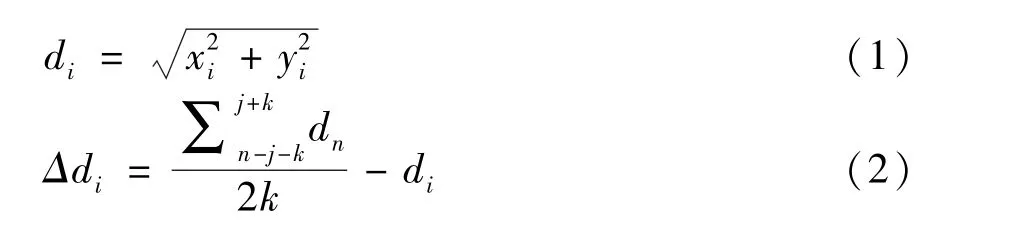
Let(xi,yi) represent theith point coordinate inXOYplane, wheredirepresents theith point distance to the origin, andkrepresents the number of neighbourhood points participating the distance variance calculation.

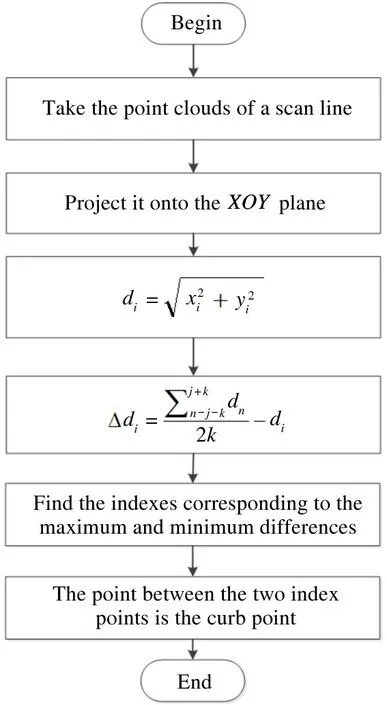
Fig.2 Flow chart of the curb annotation algorithm

Fig.3 is an example of the curb annotation algorithm. Fig.3(a) is one Lidar scan line. The points in the black box are roughly curb points. Fig.3(b) shows the distance variance of each point on the line according to Eq.(2). The maximum and the minimum are marked out in Fig.3(c) and they are selected as curb end points, which are consistent with those in the black box in Fig.3(a). After curb ends are found, all the curb points are marked. For this example, the indexes marked are 685 and 659, andkis selected as 30.

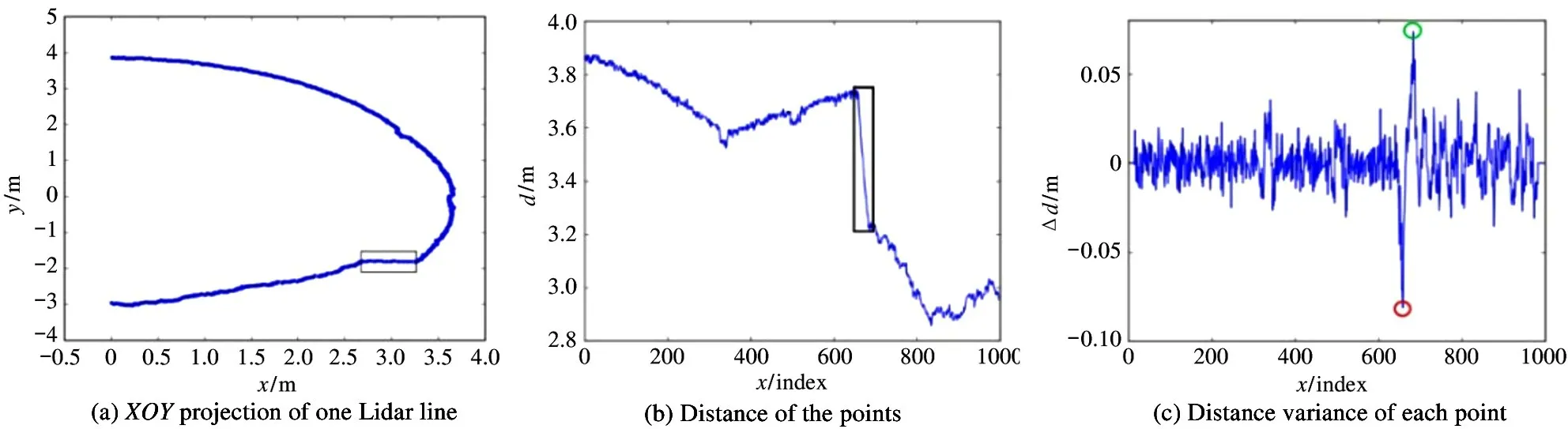
Fig.3 An example of the curb annotation algorithm

1.2 Algorithm applications in different scenarios

The algorithm performances are verified in different scenarios. The road scenarios include straight roads,curve roads,and intersections. Each scenario is considered with and without obstacles.

Fig.4 illustrates the curb annotation results.Fig.4(a) depicts results for a straight road. It is seen that curb points have been detected correctly.Fig.4(b) shows results on a curved road. The results validate algorithm robustness to different road shapes.Fig.4(c) shows the curb detection on intersections.Lidar points are sparser in this case compared with straight or curved roads. The algorithm still detects the curb points well. Fig.4(d) shows results for a road with obstacles. It is seen that some points from the obstacle are identified as curb points. The distance jump from the ground to the obstacle is captured by the algorithm while the real curb distance jump is missed.

Fig.4 The curb annotation results

In order to investigate the problem in Fig.4(d),Fig.5(a) shows theXOYprojection of a scan line point cloud with obstacles, where obstacle points and the curb points are in boxes. Fig.5(b) is the distance variance of each point calculated using Eq.(2). The maximum and the minimum variance points are marked out in circles in Fig.5(b). Two circles on the left are the maximum and the minimum variance curb points,and two circles on the right are the maximum and the minimum variance of this scan. According to the selection criteria, those two circles on the left are selected instead of the right ones. This explains why the obstacle points are mistaken as curb points.

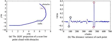
Fig.5 The curb annotation results

Once the reason is disclosed, distance variance thresholds are set to avoid the influence of the variance change from obstacles. Namely, variances beyond the thresholds are disabled. Fig.6(b) is the detection result according to this modification. It shows that the curb points are properly selected in the presence of obstacles. If the size of obstacles is large and curb points are completely blocked by obstacles, a possible curb portion may be left out.

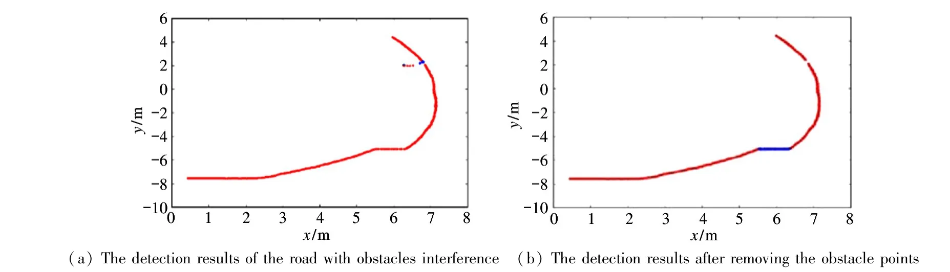
Fig.6 Detection results of curb points

This algorithm is used for labelling. Besides this,careful manual inspection is also applied. As a result,a reliable training dataset is then built for neural network training. The details on this dataset are explained in the next section.

1.3 Dataset preparation

The curb annotation algorithm is used to classify the curb points and non-curb points to generate data samples. Letg= (g1,g2, …,gn) denote a set of detected points, wheregi= (p,n,l),i= 1,2,…,n.p= (px,py,pz) represents 3D coordinates of the detected point.n=(nx,ny,nz) is the normal vector of the detected point.lis the label of the detected point,where ‘0’ represents non-curb points and ‘1’ represents curb points. Fig.7 shows a few lines of the data samples.

All the data are stored in H5 file format that is compact for data storage and is commonly used for point cloud datasets . The curb dataset built consists of 25 ×200 ×4040 points,10% of which are curb points and the rest are non-curb points.

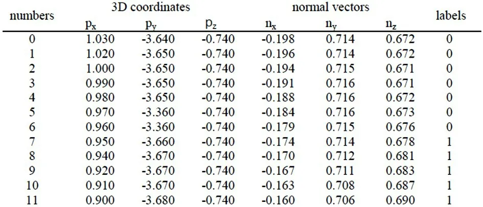
Fig.7 Data samples

1.4 EdgeNet model

The purpose of EdgeNet is to discriminate curb points from non-curb points. The backbone of the PointNet model is adopted for EdgeNet, using shared multi-layer perceptron (MLP) and max pooling to accommodate the permutation of cloud points. Fig.8 is the EdgeNet architecture. Ann×6 point cloud is input to the neural network, which containsnnumber of points and each point contains 6 features, as explained in subsection 2.3.

Fig.8 EdgeNet model structure

Firstly,n× 6 input points are passed through shared MLPs with neurons numbers for each layer defined as (64,64), which outputs ann×64 feature matrix. Next, thisn× 64 matrix is furtherly passed through shared MLP with layer neurons numbers as(64,128, 1024), and generates ann×1024 feature matrix, which is considered as expanded local features. Max pooling and average pooling are executed afterwards, which generates two 1024-dimensional global features. The next part is the fully connected layer and outputs two 128-dimensional vectors. The two 128-dimensional global features are concatenated and a 256-dimensional global feature is obtained.

For the final segmentation part, the 256-dimensional global feature is attached to each of then×1024 local feature, which generates a feature matrix with a dimension ofn×1280. Thisn×1280 matrix is then passed through another shared MLPs. Finally, two segmentations are generated for curb points and non-curb points.

2 Experiments and results

Comparison experiments are implemented in this section. Results from PointNet and DGCNN are compared with EdgeNet. All three networks are trained under the same conditions.

2.1 Training configuration

LetPoveralldenote the model overall detection accuracy as shown in Eq.(3). And curb detection accuracyPedgeis to evaluate the curb detection efficiency of the networks, which is defined in Eq.(4).

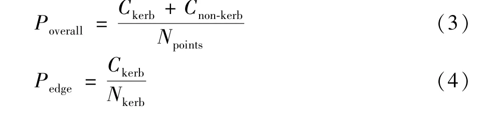
In most of the cases, curb points are the minority among all the points. For example, in the dataset,curb points are about 10% whereas non-curb points are about 90%. Curb detection accuracyPedgeis used to depict how many curb points are correctly identified among all the curb points instead of all the points.

2.2 Training results

EdgeNet training results are shown in Fig.9 and Fig.10. And the training epoch is set as 50. Fig.9 shows overall training accuracyPoveralland training loss.It is seen that EdgeNet’s final overall accuracyPoverallis around 98.4% and training loss is around 0.0417.

Fig.9 EdgeNet training results

The curb detection accuracyPedgeof each training cycle is shown in Fig.10. It is seen that EdgeNet curb detection accuracy is about 89.4%.

Fig.10 EdgeNet curb detection accuracy Pedge

2.3 Comparison experiments

In this section, PointNet and DGCNN are trained for comparison. Both PointNet and DGCNN are end-toend networks. DGCNN considers point segmentation from the graph point of view. Training and testing are performed under the same conditions for all three networks.

Table 1 shows the comparison training results.The comparison results include the training cycle number,the training time in hours, the model overall accuracyPoveralland the curb detection accuracyPedge.

Table 1 Comparison results for EdgeNet, PointNet and DGCNN

It is seen from Table 1 and Fig.11 that EdgeNet is better in the curb detection accuracy, which is about 5% higher than PointNet and about 1% higher than DGCNN. Subsection 2.4 compares the curb detection results in different scenarios.

Fig.11 Curb detection accuracy Pedge

2.4 Test results in different scenarios

Fig.12 Comparisons of curb detection results in a straight road

Fig.13 Comparisons of curb detection results in a curve road

Fig.14 Comparisons of curb detection results in an intersection

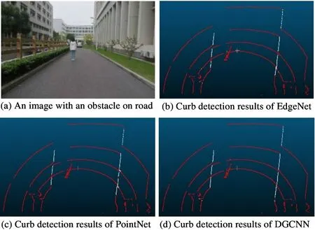
Fig.15 Comparisons of curb detection results in a road with obstacles

Figs12 -15 show the comparisons results for four different road scenarios, including straight roads,curve roads, intersections and roads with obstacles.Three methods (EdgeNet, PointNet and DGCNN), are tested. Table 2 summarizes the detection accuracies of these three methods in four scenarios, includingPoverallandPedge.It is seen that all the methods can effectively detect the curb points, and theirPoverallaccuracies are above 95%. And EdgeNetPedgeaccuracies are the highest, which means its ability to detect curbs is the best among them.

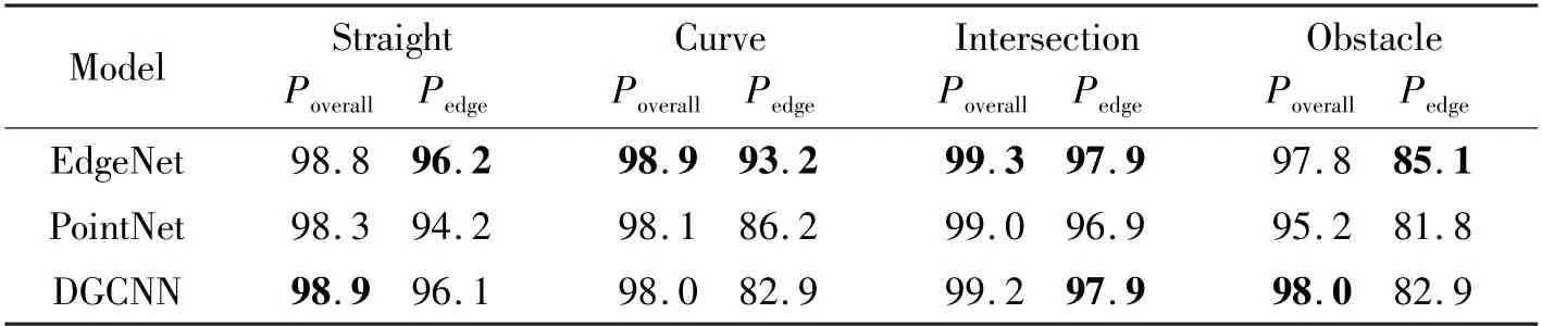
Table 2 Comparison results for different scenarios (%)

3 Conclusions

In this work,an end-to-end deep learning network(EdgeNet) is proposed for curb detection, which handles Lidar cloud points directly. EdgeNet marks out curb points in the output. A curb annotation algorithm is also designed to generate dataset for training EdgeNet. Overall, this neural network method avoids tedious manual parameter adjustments and provides good segmentation of curb points and non-curb points under different road scenarios. The comparison results of Edgenet, PointNet and DGCNN are also provided. Comparatively, EdgeNet learns curb features for curb segmentation better, which has been validated in the experiments.