Multi-layer dynamic and asymmetric convolutions①

LUO Chunjie (罗纯杰), ZHAN Jianfeng

(Institute of Computing Technology, Chinese Academy of Sciences, Beijing 100190, P.R.China)

(University of Chinese Academy of Sciences, Beijing 100049, P.R.China)

Abstract Dynamic networks have become popular to enhance the model capacity while maintaining efficient inference by dynamically generating the weight based on over-parameters. They bring much more parameters and increase the difficulty of the training. In this paper,a multi-layer dynamic convolution (MDConv) is proposed, which scatters the over-parameters over multi-layers with fewer parameters but stronger model capacity compared with scattering horizontally; it uses the expanding form where the attention is applied to the features to facilitate the training; it uses the compact form where the attention is applied to the weights to maintain efficient inference. Moreover, a multi-layer asymmetric convolution (MAConv) is proposed,which has no extra parameters and computation cost at inference time compared with static convolution. Experimental results show that MDConv achieves better accuracy with fewer parameters and significantly facilitates the training;MAConv enhances the accuracy without any extra cost of storage or computation at inference time compared with static convolution.

Key words: neural network, dynamic network, attention, image classification

0 Introduction

Deep neural networks have received great successes in many areas of machine intelligence. Many researchers have shown rising interest in designing lightweight convolutional networks[1-8]. Light-weight networks improve the efficiency by decreasing the size of the convolutions. That also leads to the decrease of the model capacity.

Dynamic networks[9-12]have become popular to enhance the model capacity while maintaining efficient inference by applying attention on the weight. Conditionally parameterized convolutions (CondConv)[9]and dynamic convolution (DYConv)[10]were proposed to use a dynamic linear combination ofnexperts as the kernel of the convolution. CondConv and DYConv bring much more parameters. WeightNet[11]used a grouped fully-connected layer applied to the attention vector to generate the weight in a group-wise manner,achieving comparable accuracy with fewer parameters than CondConv and DYConv. Dynamic convolution decomposition (DCD)[12]replaced dynamic attention over channel groups with dynamic channel fusion, resulting in a more compact model. However, DCD brings new problems: it increases the depth of the weight, thus it hinders error back-propagation; it increases the dynamic coefficients since it uses a full dynamic matrix. More dynamic coefficients make the training more difficult.

To reduce the parameters and facilitate the training, a multi-layer dynamic convolution (MDConv) is proposed, which scatters the over-parameters over multi-layers with fewer parameters but stronger model capacity compared with scattering horizontally; it uses the expanding form where the attention is applied to the features to facilitate the training; it uses the compact form where the attention is applied to the weights to maintain efficient inference. In CondConv and DYConv, the over-parameters are scattered horizontally.The key foundation for the success of deep learning is that deeper layers have stronger model capacity. Unlike CondConv and DYConv, MDConv scatters overparameters over multi-layers, enhancing the model capacity with fewer parameters. Moreover, MDConv brings fewer dynamic coefficients thus is easier to train compared with DCD. There are two additional mechanisms to facilitate the training of deeper layers in the expanding form. One is batch normalization (BN) after each convolution. BN can significantly accelerate and improve the training of deeper networks. The other mechanism that helps the training is the bypass convolution with the static kernel. The bypass convolution shortens the path of error back-propagation.

At training time, the attention in MDConv is applied to features. While at inference time,the attention becomes weight attention. Batch normalization can be fused into the convolution. Squeeze-and-excite (SE)attention can be viewed as a diagonal matrix. Then,the three convolutions and SE attention can be further fused into a single convolution with dynamic weight for efficient inference. After fusion, the weight of the final convolution for inference is dynamically generated, and only one convolution needs to be performed. When implementing, there is no need to construct the diagonal matrix. After generating the dynamic coefficients,broadcasting multiply can be used instead of matrix multiply. Thus MDConv costs fewer memories and computational resources than DCD, which generates a dense matrix.

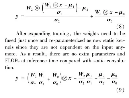
Although dynamic attention could significantly enhance the model capacity, it brings extra parameters and the number of float point operations (FLOPs) at inference time. Besides multi-layer dynamic convolution, a multi-layer asymmetric convolution (MAConv)is proposed, which removes the dynamic attention from multi-layer dynamic convolution. After the training,the weights need to be fused just one time and re-parameterized as new static kernels since they do not depend on the input anymore. As a result, there are no extra parameters and FLOPs at inference time compared with static convolution.

The experiments show that:

The remainder of this paper is structured as follows. Section 1 briefly presents related work. Section 2 describes the details of multi-layer dynamic convolution. Section 3 introduces multi-layer asymmetric convolution. In Section 4, the experiment settings and the results are presented. Conclusions are made in Section 5.

1 Related work

1.1 Dynamic networks

CondConv[9]and DYConv[10]compute convolutional kernels as a function of the input instead of using static convolutional kernels. In particular,the convolutional kernels are over-parameterized as a linear combination ofnexperts. Although largely enhancing the model capacity, CondConv and DYConv bring much more parameters, thus are prone to over-fitting. Besides, more parameters require more memory resources. Moreover, the dynamics make the training more difficult. To avoid over-fitting and facilitate the training, these two methods apply additional constraints. For example, CondConv shares routing weights between layers in a block. DYConv uses the Softmax with a large temperature instead of Sigmoid on the output of the routing network. WeightNet[11]uses a grouped fully-connected layer applied to the attention vector to generate the weight in a group-wise manner.WeightNet achieves comparable accuracy with fewer parameters than CondConv and DYConv. To further compact the model, DCD[12]decomposes the convolutional weight, which reduces the latent space of the weight matrix and results in a more compact model.

Although dynamic weight attentions enhance the model capacity, they increase the difficulty of the training since they introduce dynamic factors. Extremely, dynamic filter network[13]generates all the convolutional filters dynamically conditioned on the input. On the other hand, SE[14]is an effective and robust module by applying attention to the channel-wise features.Other dynamic networks[15-20]try to learn dynamic network structure with static convolution kernels.

1.2 Re-parameterization

ExpandNet[21]expands convolution into multiple linear layers without adding any nonlinearity. The expanding network can benefit from over-parameterization during training and can be compressed back to the compact one algebraically at inference. For example, ak×kconvolution is expanded by three convolutional layers with kernel size 1 ×1,k×kand 1 ×1, respectively. ExpandNet increases the network depth, thus makes the training more difficult. ACNet[22]uses asymmetric convolution to strengthen the kernel skeletons for powerful networks. At training time, it uses three branches with 3 ×3, 1 ×3, and 3 ×1 kernels respectively. At inference time, the three branches are fused into one static kernel. RepVGG[23]constructs the training-time model using branches consisting of identity map, 1 ×1 convolution and 3 ×3 convolution. After training, RepVGG constructs a single 3 ×3 kernel by re-parameterizing the trained parameters. ACNet and RepVGG can only be used fork×k(k ＞1) convolution.

2 Multi-layer dynamic convolution

The main problem of CondConv[9]and DYConv[10]is that they bring much more parameters. DCD[12]reduces the latent space of the weight matrix by matrix decomposition and results in a more compact model.However, DCD brings new problems: (1) it increases the depth of the weight, thus hinders error back-propagation; (2) it increases the dynamic coefficients since it uses a full dynamic matrix. More dynamic coefficients make the training more difficult. In the extreme situation, e. g., dynamic filter network[13], all the convolutional weights are dynamically conditioned on the input. It is hard to train and can not be applied in modern deep architecture successfully.

To reduce the parameters and facilitate the training, MDConv is proposed. As shown in Fig.1, MDConv has two branches: (1) the dynamic branch consists of ak×k(k ＞= 1) convolution, a SE module,and a 1 ×1 convolution; (2) the bypass branch consists of ak×kconvolution with a static kernel. The output of MDConv is the addition of the two branches.

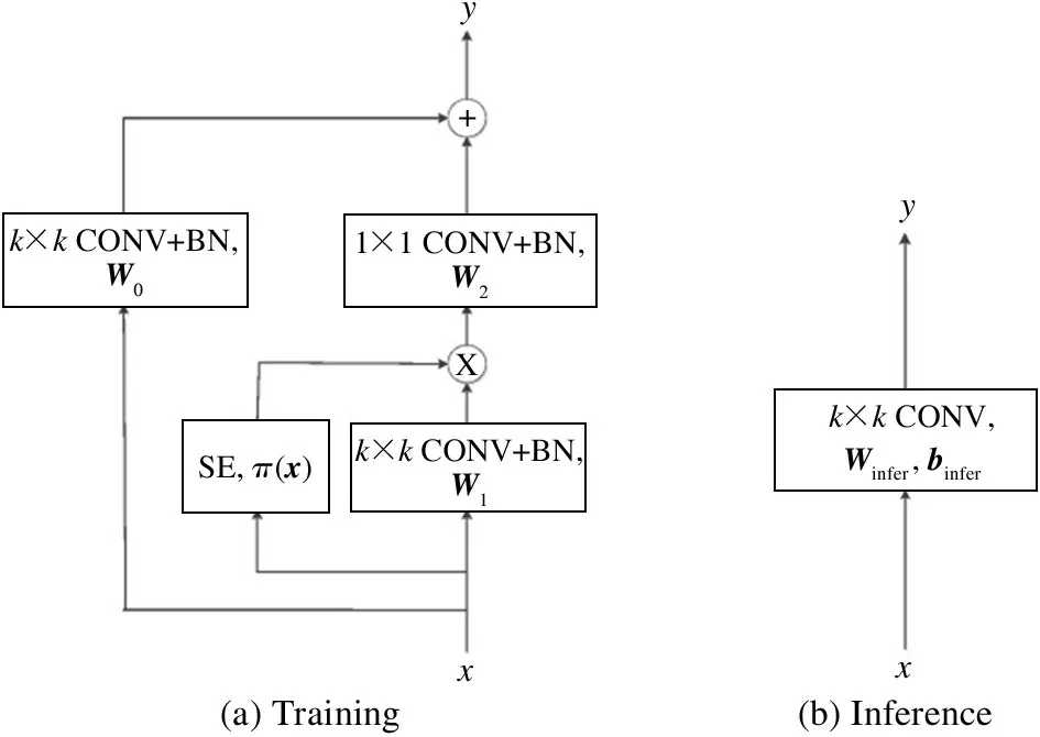
Fig.1 Training and inference of MDConv

Unlike CondConv and DYConv, MDConv encapsulates the dynamic information into multi-layer convolutions by applying SE attention between two convolutional layers. By scattering the over-parameters over multi-layers, MDConv increases the model capacity with fewer parameters than horizontally scattering. Moreover, MDConv facilitates the training of dynamic networks. In MDConv, SE can be viewed as a diagonal matrixA.

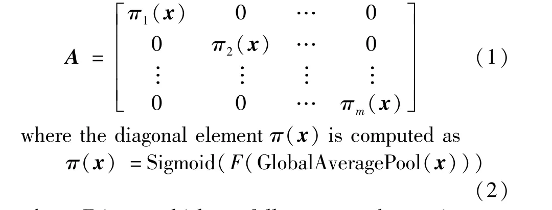
whereFis a multi-layer fully-connected attention network. Compared with DCD, which uses a full dynamic matrix, MDConv brings fewer dynamic coefficients thus is easier to train. There are two additional mechanisms to facilitate the training of deeper layers in MDConv.One is batch normalization after each convolution.Batch normalization can significantly accelerate and improve the training of deeper networks. Another mechanism that helps the training is the bypass convolution with the static kernel. The bypass convolution shortens the path of error back-propagation.

MDConv uses two layer convolutions in the dynamic branch. Three or more layers bring the following problems: (1) more convolutions bring more computation FLOPs; (2) more dynamic layers are harder to train and need more training data.

Although the expanding form of MDConv facilitates the training, it is more expensive since there are three convolutional operators at training time. The compact form of MDConv can be used for efficient inference. MDConv can be defined as

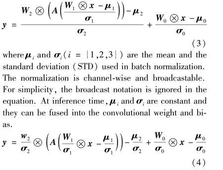
Then the three convolutions of MDConv can be fused into a single convolution for efficient inference.

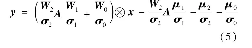
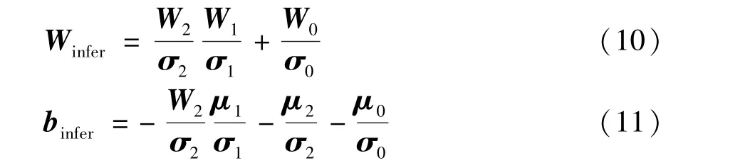
whereWinferandbinferare the new weight and bias of the convolution after re-parameterization.

When implementing, the diagonal matrixAdoes not need be constructed. After generating the dynamic coefficients, the broadcasting multiply can be used instead of matrix multiply. Thus MDConv costs fewer memories and computational resources than DCD,which generates a dense matrixA.

3 Multi-layer asymmetric convolution

Although dynamic attention could significantly enhance model capacity, it still brings extra parameters and FLOPs at inference time. Besides MDConv, this paper also proposes MAConv, which removes the dynamic attention in MDConv.

In ExpandNet[21], ak×k(k＞=1) convolution is expanded vertically by three convolutional layers with kernel size 1 × 1,k×k, 1 × 1, respectively.Whenk ＞1,it cannot use BN in the intermediate layer. The bias caused by BN fusion cannot pass forward through thek×kkernel, thus cannot be fused with the bias of the next layer. MAConv avoids this problem,thus can use BN to facilitate the training. Besides,MAConv uses the bypass convolution for shortening the path of error back-propagation. BN and the bypass shortcut in MAConv help the training of deep layers.Both BN and the bypass shortcut can be compressed and re-parameterized to the compact one, thus without any extra cost at inference time.

ACNet[22]and RepVGG[23]horizontally expand thek×k(k ＞1) convolution into convolutions with different kernel shape. That hinders its usage for lightweight networks, which heavily utilizes the 1 ×1 pointwise convolutions. MAConv uses asymmetric depth instead of asymmetric kernel shape and expands the convolution both vertically and horizontally. MAConv can be used for both 1 ×1 convolution andk×k(k ＞1)convolution.

4 Multi-layer asymmetric convolution

4.1 ImageNet

ImageNet classification dataset[24]has 1.28 ×106training images and 50 000 validation images with 1000 classes. The experiments are based on the official example of Pytorch.

The standard augmentation is used for training image as the same as the official example: (1) randomly cropped with the size of 0.08 to 1.0 and aspect ratio of 3/4 to 4/3, and then resized to 224 ×224; (2) randomly horizontal flipped. The validation image is resized to 256 ×256, and then center cropped with size 224 ×224. Each channel of the input image is normalized into 0 mean and 1 STD globally. The batch size is 256. Four TITAN Xp GPUs are used to train the models.

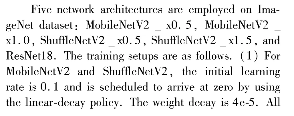
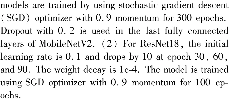
Firstly, comparisons are made between static convolution, DYConv[10], MAConv, and MDConv on MobileNetV2 and ShuffleNetV2. For DYConv, the number of experts is set to the default value 4[10]. For MDConv and MAConv, the number of intermediate channelsmis set to 20. For DYConv and MDConv, the attention network is a two-layer fully-connected network with the hidden units to be 1/4 input channels. As recommended in the original paper[10], the temperature of Softmax is set to 30 in DYConv. DYConv, MDConv, and MAConv are applied to the pointwise convolutional layer in the inverted bottlenecks of Mobile-NetV2 or the blocks of ShuffleNetV2. They are used to replace the static convolution.

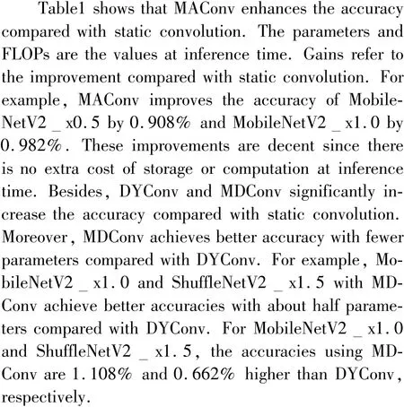
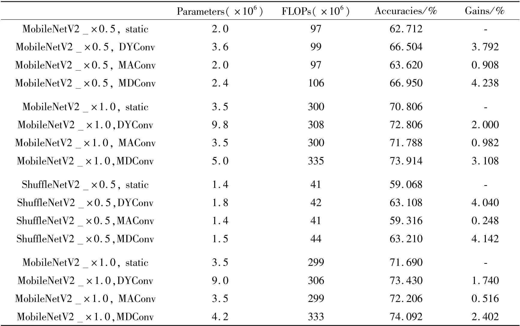
Table 1 Top-1 accuracies of lightweight networks on ImageNet validation dataset

Comparisons are also made onk×k(k ＞1) convolution. DYConv, MDConv, and MAConv are applied in the 3 ×3 convolutional layer of ResNet18’s residual block. Table 2 shows that MAConv is also effective onk×k(k ＞1) convolution. MDConv increases the accuracy by 2.086% with only 1 ×106additional parameters compared with static convolution. Moreover, it achieves higher accuracy with much fewer parameters than DYConv.

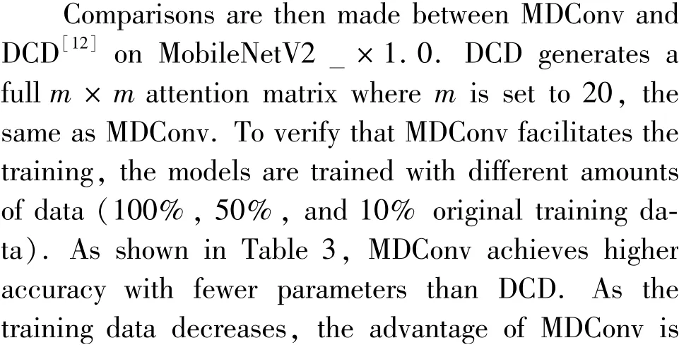
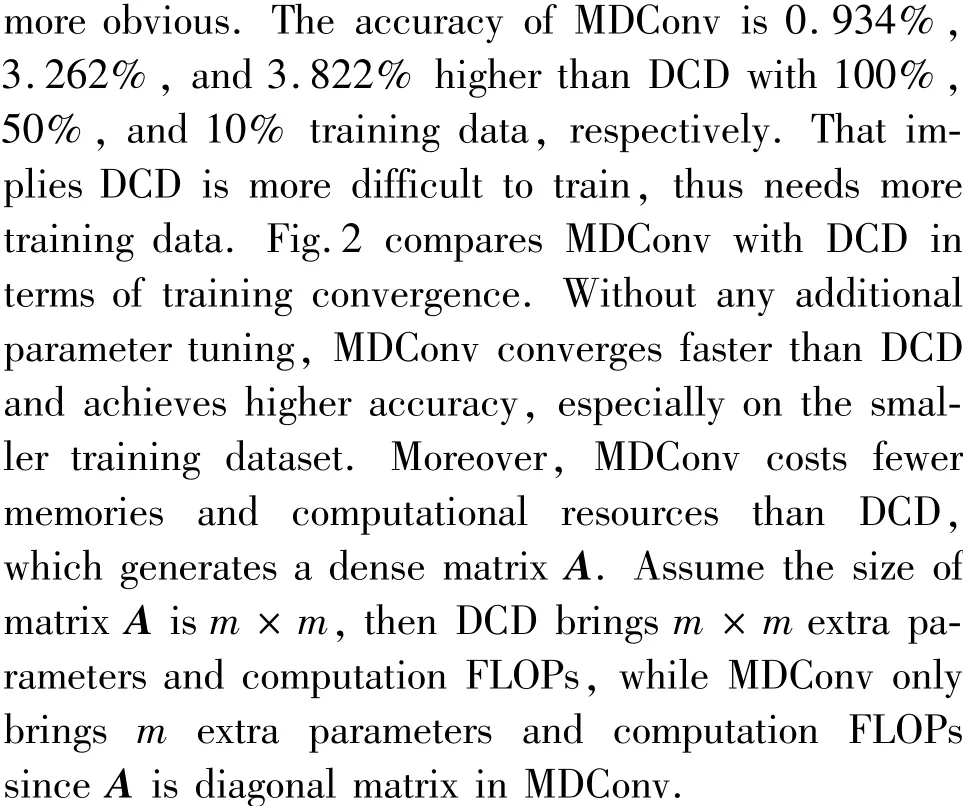
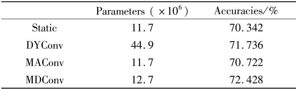
Table 2 Top-1 accuracies of ResNet18 on ImageNet validation dataset

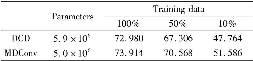
Table 3 Comparison of validation accuracies (%) between DCD and MDConv on MobileNetV2x1. 0 trained with different amounts of data

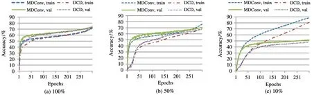
Fig.2 Comparison of training and validation accuracy curves between DCD and MDConv on MobileNetV2x1.0 trained with different amounts of data

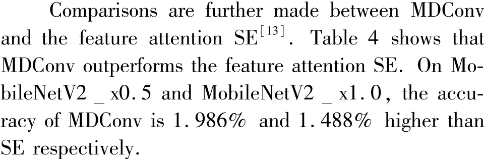
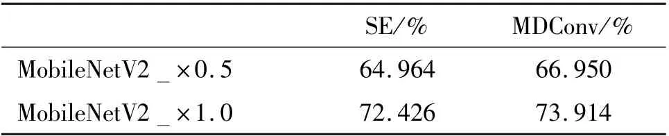
Table 4 Comparison of validation accuracies on ImageNet between MDConv and SE

4.2 CIFAR-10

CIFAR-10 is a dataset of natural 32 ×32 RGB images in 10 classes with 50 000 images for training and 10 000 for testing. The training images are padded with 0 to 36 ×36 and then randomly cropped to 32 ×32 pixels. Then randomly horizontal flipping is made. Each channel of the input is normalized into 0 mean and 1 STD globally.

SGD with momentum 0.9 and weight decay 5e-4 are used. The batch size is set to 128. The learning rate is set to 0.1, and scheduled to arrive at zero using the cosine annealing scheduler. The networks are trained with 200 epochs.

MobileNetV2 with different width multipliers are evaluated on this small dataset. The setups for different attentions are the same as subsection 4.1. Each test is run 5 times. The mean and the STD of the accuracies are listed in Table 5. MAConv increases the accuracy compared with static convolution. MAConv even outperforms DYConv on this small dataset. MDConv further improves the performance and achieves the best performance, while DCD achieves the worst performance and has large variance. That implies again DCD brings more dynamics and is difficult to train on the small dataset.

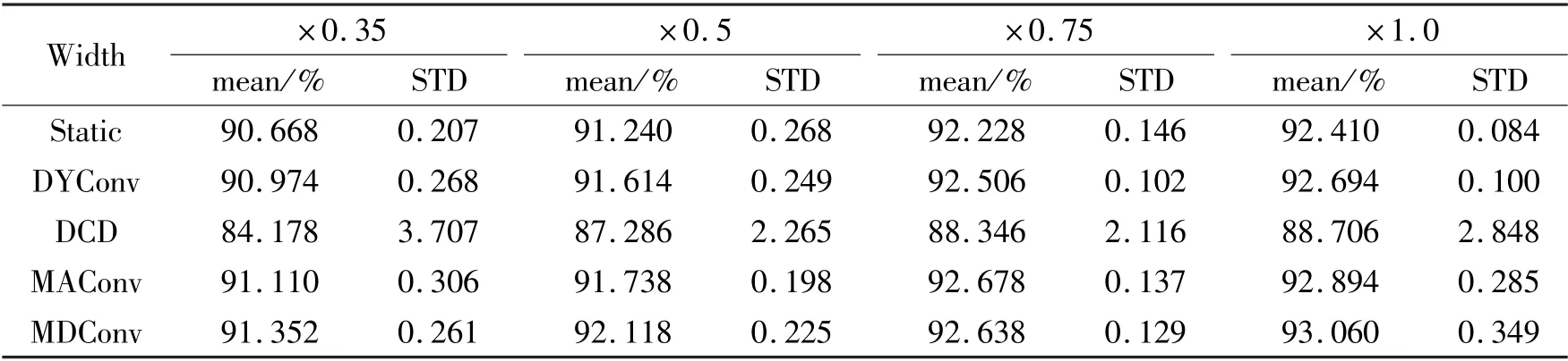
Table 5 Test accuracies on CIFAR-10 with MobileNetV2

4.3 CIFAR-100

CIFAR-100 is a dataset of natural 32 ×32 RGB images in 100 classes with 50 000 images for training and 10 000 for testing. The training images are padded with 0 to 36 ×36 and then randomly cropped to 32 ×32 pixels. Then randomly horizontal flipping is made.Each channel of the input is normalized into 0 mean and 1 STD globally. SGD with momentum 0. 9 and weight decay 5e-4 are used. The batch size is set to 128. The learning rate is set to 0.1, and scheduled to arrive at zero using the cosine annealing scheduler.The networks are trained with 200 epochs.

MobileNetV2x0.35 is evaluated on this dataset.The setups for different attentions are the same as subsection 4.1. Each test is run 5 times. The mean and the standard deviation of the accuracies are reported in Table 6. Results show that dynamic networks do not improve the accuracy compared with the static network. Moreover, more dynamic factors lead to worse performance. For example, DCD is worse than MDConv, and MDConv is worse than DyConv. That is because dynamic networks are harder to train and need more training data and CIFAR-100 has 100 classes,and each class has fewer training examples than CIFAR-10.MAConv achieves the best performance, 70. 032%.When the training dataset is small, MAConv is still effective to enhance the model capacity instead of dynamic ones.

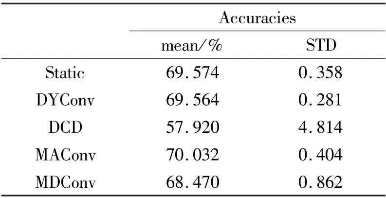
Table 6 Test accuracies on CIFAR-100

4.4 SVHN

The street view house numbers (SVHN) dataset includes 73 257 digits for training, 26 032 digits for testing, and 531 131 additional digits. Each digit is a 32 ×32 RGB image. The training images are padded with 0 to 36 ×36 and then randomly cropped to 32 ×32 pixels. Then randomly horizontal flipping is made.Each channel of the input is normalized into 0 mean and 1 STD globally. SGD with momentum 0.9 and weight decay 5e-4 are used. The batch size is set to 128. The learning rate is set to 0.1, and scheduled to arrive at zero using the cosine annealing scheduler. The networks are trained with 200 epochs.

MobileNetV2x0.35 is used on this dataset. The setups for different attentions are the same as subsection 4.1. Each test is run 5 times. The mean and the standard deviation of the accuracies are reported in Table 7. Results show that DCD decreases the performance compared with the static one. DCD is hard to train on the small dataset. DYConv, MAConv, and MDConv increase the accuracy compared with the static one. Among them, MAConv and MDConv achieve similar performance, better than DYConv.

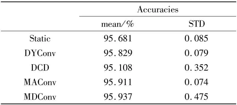
Table 7 Test accuracies on SVHN

4.5 Ablation study

Ablation experiments are carried out on CIFAR-10 using two network architectures. One is MobileNetV2 x0.35. To make the comparison more distinct, a smaller and simpler network named SmallNet is also used.SmallNet has the first convolutional layer with 3 × 3 kernels and 16 output channels, followed by three blocks. Each block comprises of a 1 ×1 pointwise convolution with 1 stride and no padding, and a 3 × 3 depthwise convolution with 2 strides and 1 padding.These 3 blocks have 16, 32 and 64 output channels,respectively. Each convolutional layer is followed by batch normalization, and ReLU activation. The output of the last layer is passed through a global average pooling layer, followed by a Softmax layer with 10 classification output. Other experiment settings are the same as subsection 4.2.

The effect of the bypass shortcut in the MAConv and MDConv is investigated firstly. To show the effect of dynamic attention, ReLU activation is further used instead of dynamic attention in the multi-layer branch.The results are shown in Table 8, w/ means with bypass shortcut, w/o means without bypass shortcut. Results show that the bypass shortcut improves the accuracy, especially in deeper networks (MobileNetV2 x0.35). Moreover, MDConv (with dynamic attention)increases the capabilities of models compared with MAConv (without dynamic attention). Using ReLU activation instead of dynamic attention can further increase the capabilities. However, the weights cannot be fused into compact one anymore because of the non-linear activation function. Thus the costs of storage and computation are much higher than single-layer convolution at inference time.

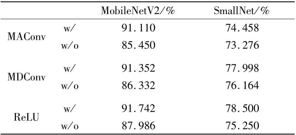
Table 8 Effect of bypass shortcut

Next, the networks are trained by using the compact form directly. Table 9 shows the comparison between the expanding training and the compact training.Results show that expanding training improves the performance of MAConv and MDConv. To evaluate the benefit of BN in expanding training, BN is applied after the addition of two branches instead of after each convolution (without BN after each convolution). Resultsshow that BN in expanding form helps the training since it achieves better performance than that without BN. Moreover, the expanding form without BN helps training itself, since it achieves better performance than compact training.

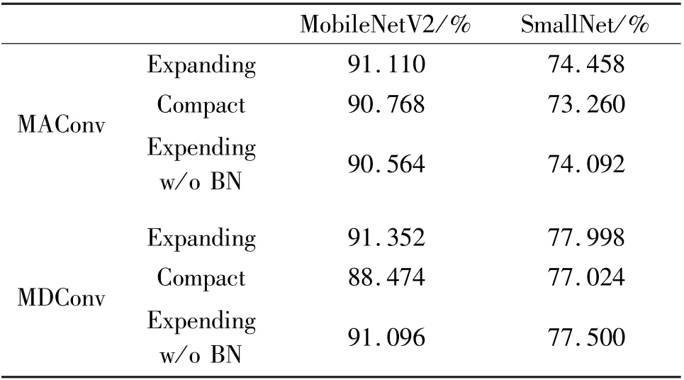
Table 9 Effect of expanding training

The effect of different input/output channels and different intermediate channels are also investigated.Different width multipliers are applied on all layers except the first layer of SmallNet. The results are shown in Table 10. Results show that the gains of MAConv and MDConv are higher with fewer channels. These results imply that over-parameterization is more effective in smaller networks. SmallNet are then trained with different intermediate channels. The results are shown in Table 11. Results show that the gains of MAConv and MDConv are trivial when increasing the intermediate channel on the CIFAR-10 dataset. Using more intermediate channels means that the dynamic part takes more influence, thus increases the difficulty of training and needs more training data.

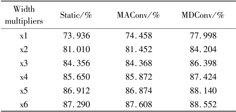
Table 10 Effect of input/output channel width

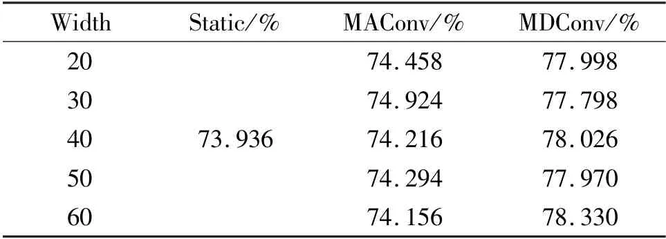
Table 11 Effect of different intermediate channel width

Finally, different setups for the attention network are investigated in SmallNet with MDConv. Different numbers of the hidden units are used, ranging from 1/4 times of the input channel to 4 times of the input channel. Table 12 shows that increasing hidden units can improve the performance until 4 times of the input channel. Softmax and Softmax with different temperatures, as proposed in Ref.[10], are used as the gate function in the last layer of the attention network. As shown in Table 13, Softmax achieves better accuracy than Sigmoid. However, the temperature does not improve the performance.

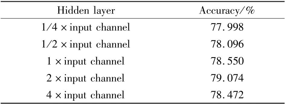
Table 12 Effect of the hidden layer in the attention network

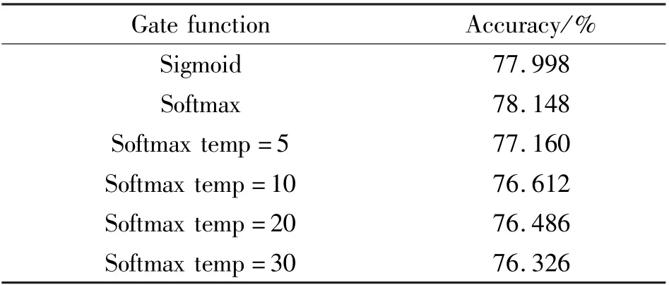
Table 13 Effect of the gate function in the last layer of the attention network

5 Conclusions

Two powerful convolutions are proposed to increase the model’s capacity: MDConv and MAConv.MDConv expands the static convolution into multi-layer dynamic one, with fewer parameters but stronger model capacity than horizontally expanding. MAConv has no extra parameters and FLOPs at inference time compared with static convolution. MDConv and MAConv are evaluated on different networks. Experimental results show that MDConv and MAConv improve the accuracy compared with static convolution. Moreover,MDConv achieves better accuracy with fewer parameters and facilitates the training compared with other dynamic convolutions.