Nonrecursive residual Monte Carlo method for SN transport discretization error estimation

Yun-Huang Zhang

Abstract In this paper,we present a nonrecursive residual Monte Carlo method for estimating discretization errors associated with the SN transport solution to radiation transport problems. Although this technique is general, we applied it to the mono-energetic 1-D SN equation with linear-discontinuous finite element method spatial discretization as a demonstration of the theory for the purpose of this study.Two angular flux representations:conforming and simplified representations were considered in this analysis, and the results were compared. It is shown that the simplified representation dramatically reduces the memory footprint and computational complexity of residual source generation and sampling while accurately capturing the error associated with certain types of responses.

Keywords Residual Monte Carlo · Discretization error ·Angular flux representation

1 Introduction

Efficient and accurate solutions to the radiation transport equation are of fundamental importance in the simulation of fission reactor cores, nuclear fusion, and radiation shielding. The Monte Carlo method [1] and deterministic methods (such as SN[2, 3], PN[4], and SPN[5–9]) are two different approaches to the solution of the transport equation. The Monte Carlo method is capable of producing fairly accurate results at the cost of an enormous amount of CPU hours, whereas deterministic methods can be performed at a fraction of the cost but often suffer from model errors and discretization errors. Several efforts have been made to combine these two methods to achieve better efficiency and accuracy. One of them falls in the residual Monte Carlo category [10, 11], where the deterministic method is invoked recursively to accelerate the convergence of the Monte Carlo calculation[12–14].On the other hand, one can also start with a deterministic solution and use Monte Carlo to perform error correction.This new idea is a nonrecursive approach and is expected to exhibit superior performance in problems for which coarse-mesh deterministic calculations are capable of capturing the fundamental structure of the solution.

Consider the mono-energetic 1-D neutron transport equation with the Legendre scattering cross-sectional expansion truncated at order L. For simplicity, we assume an isotropic distributed source:

where m is the discrete direction index running from 1 to M and M is the total number of directions. Along each direction, a first-order ordinary differential equation is solved using a spatial discretization technique such as discontinuous finite element method [15, 16]. The equations along different directions are coupled through the scattering term. The ～in Eq. (2) indicates that the SNsolution is an approximation of the true transport solution,in the sense that the SNsolution is subject to angular and spatial discretization errors.In the pursuit of a high-fidelity simulation, it is often desirable to estimate the discretization error,given an approximate solution.This process can be computationally costly because it generally entails mesh refinements in a high-dimensional phase space(in this case,space and angle). The required computation can become prohibitively expensive when the dimensionality is high and/or the solution does not exhibit adequate regularity,which can lead to convergence degradation.

We propose a novel approach to tackle this challenge using the Monte Carlo method to evaluate the deterministic numerical error. Let us first rewrite the transport equation in operator form as

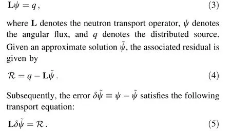
We emphasize that L needs to be the true transport operator for Eq. (5) to hold. To numerically solve for δ～ψ, it might be tempting to substitute L with a high-order deterministic transport operator, such as SN, projected onto a highly refined space-angle mesh.However,as stated earlier in this section, this is computationally expensive. The key to this approach is to use the Monte Carlo method to invert L,which is inherently exempt from discretization errors. The residual Monte Carlo method presented here is significantly more efficient than the standard Monte Carlo method,where the full solution is first calculated,and then,the error is computed by subtracting the deterministic solution from the Monte Carlo solution.This is because the residual Monte Carlo method directly computes the error itself and concentrates computational resources toward phase-space regions where the residual is large by sampling source particles from a probability distribution function that is proportional to the absolute value of the residual. We refer to this procedure as a nonrecursive residual Monte Carlo method to differentiate it from the standard version of the residual Monte Carlo method. The standard residual Monte Carlo method involves a recursive set of calculations combined with phase-space adaptive mesh refinement to achieve exponential convergence with the number of particle histories [17–19].

Because the residual function can change sign, a source particle sampled from its absolute value (｜R｜) carries a weight bearing the sign of the original residual function at its sampled phase-space coordinate. Another difficulty caused by changing the sign is associated with the integration of the probability distribution function over the phase space, which is an indispensable step in source sampling. More specifically, nonsmoothness across the sign-changing boundary (see Fig. 1) is problematic for numerical integration. In the case of 1-D transport calculation with linear finite element spatial representation, one can determine the sign boundary analytically and compute the integral using a divide-and-conquer approach.In multi-D, however, computing the boundary is difficult . To this end, we propose a simplified angular flux representation that is isotopic in angle and piecewise constant in space.As will be shown later in this paper, as long as the simplified representation preserves the original SNscalar flux, the resulting error estimation is exact for angle-space integrated responses such as cell-averaged scalar flux and reaction rate.

Note that, although the discussion presented in this paper revolves around mono-energetic 1-D transport calculation, the basic principle can be equally applied to multigroup multi-D transport problems.A flowchart for the entire scheme of the residual Monte Carlo method is presented in Fig. 2

The remainder of this paper is organized as follows.First, we consider the SNequation with standard lineardiscontinuous(LD)finite element spatial discretization and generate the associated residual. We then introduce a simplified spatial representation for the angular flux and explain the residual generation using this simplified representation. Next, we discuss some technical details for sampling source particles from the residual function as well as the boundary conditions and current cell interface preservation techniques. Next, we present numerical test results to demonstrate the efficacy of the method . Finally,we summarize our findings and provide recommendations for future work.

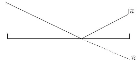
Fig. 1 Nonsmoothness in the absolute value of R

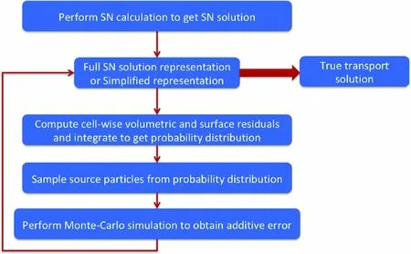
Fig. 2 Residual Monte Carlo flow chart

2 Standard linear discontinuous finite element and residual generation

The prerequisite for the residual Monte Carlo method is a functional representation of the SNangular flux,which is defined at every space-angle point.This construction is not unique. The representation presented below is relatively straightforward and conformal to the discretization scheme.

2.1 Piecewise constant angular representation

We assume that the angular flux is constant within the angle interval associated with each discrete SNdirection.That is,

2.2 Linear-discontinuous finite element method spatial discretization

Linear-discontinuous finite element method (LD-FEM)is a standard spatial discretization scheme for the first-order SNtransport equation.In this method,the spatial solution is projected onto a set of basis functions that are linearly continuous within each cell but discontinuous across cell interfaces.In particular,a pair of basis functions （BL，BR）for cell i is defined as

2.3 Residual generation with LD-FEM

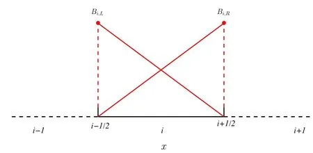
Fig. 3 Linear-discontinuous basis functions for cell i

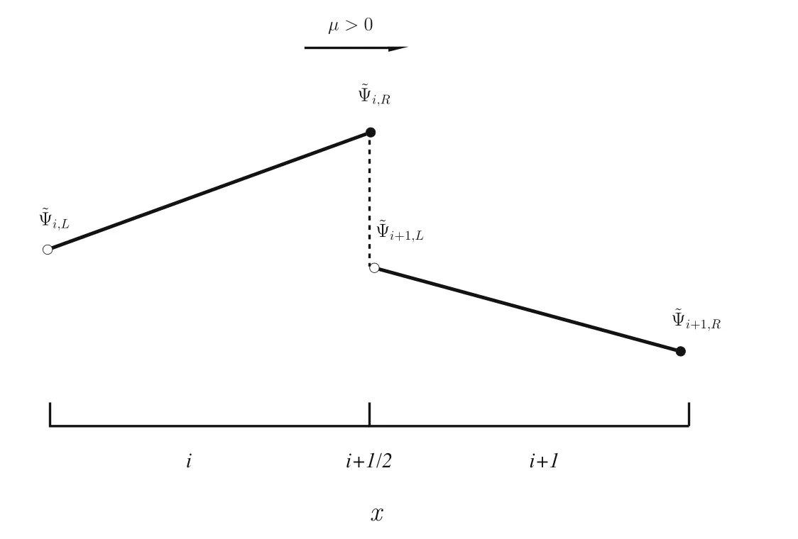
Fig. 4 Linear-discontinuous spatial representations with upwinding

In the case of LD-FEM spatial representation, the residual generation can be conveniently divided into two parts: cell-interior residual and cell-interface residual. To simplify the discussion, let us assume isotropic scattering.By substituting Eqs. (13) and (8) into Eq. (4), we obtain the cell-interior residual. In particular, for cell i and angle bin m,

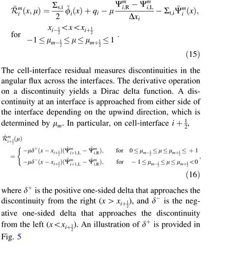
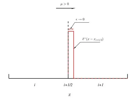
Fig. 5 Positive one-sided delta function

3 Simplified angular flux representation and residual generation

Equation (15)indicates that ～R can change sign within a phase-space cell. As will be shown in Sect. 4, the integration of the residual over each phase-space cell needs to be computed as part of the source sampling procedure. As explained in Sect. 1, the sign change within the phasespace cell poses a challenge to numerical integration schemes. Moreover, the standard conformal angular flux representation requires a solution at each spatial DoF and for each discrete direction. This requires additional memory costs, as typical SNcodes only store moment values.

3.1 Isotropic and piecewise constant angular flux representation

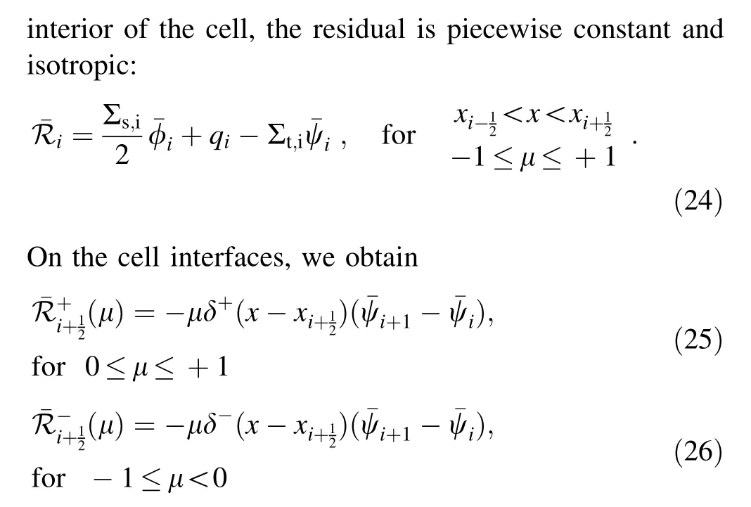
To simplify the structure of the residual and thereby simplify the source sampling procedure, we propose a simplified angular flux representation that is isotropic in angle and piece(cell)-wise constant in space. Despite the dramatic reduction in complexity, it can be shown that, as long as the simplified representation preserves the original cell-integrated scalar flux,the error estimation for the cellintegrated responses, such as cell-averaged scalar flux and reaction rate, is rigorous. The simplified angular flux representation is as follows:

An illustration of the simplified angular flux representation for μ ＞0 is provided in Fig. 6.

3.2 Residual generation with the simplified representation

Fig. 6 Isotropic and piecewise constant angular flux representations with upwinding

In this case, the cell interior residual does not change sign within a phase-space cell; therefore, the residual integration is straightforward. From the memory saving perspective, in 1-D, the simplified representation requires storing only one DoF per cell for all directions, whereas LD representation stores two DoFs per cell and for each M discrete direction. Hence, 2×M memory savings are achieved. In the case of 2-D and 3-D, the saving factor is 4×M（M+2） and 8×M（M+2）, respectively.

4 Source sampling for residual Monte Carlo

From the perspective of implementation,the only major difference between the residual Monte Carlo and standard Monte Carlo methods resides in the source sampling, after which the standard Monte Carlo algorithm can be equally applied to the residual Monte Carlo method for tracking the history of the sampled particles.Unlike the standard Monte Carlo method that samples source particles from a given source probability distribution, the residual Monte Carlo method samples particles from a distribution that is proportional to the absolute value of the residual, ｜R｜. More specifically, the residual source probability distribution is｜R｜re-normalized as follows:

In practice, a hierarchical approach is adopted. First, the angle-space cell index (m, i) or cell index (i) is sampled depending on the angular flux representation. Subsequently, the actual position and direction of the source particle are sampled from within that cell.

4.1 Discrete sampling for angle-space cell index

The angle-space cell index is sampled from a probability mass function,which is the discrete version of Eq. (27).In the case of the standard LD representation,

4.2 Sampling angle-space coordinates from within a cell

Once the angle-space cell index is determined,the actual spatial position and flight direction of the source particle can be sampled. The sampling procedure is divided between the cell interiors and the cell interfaces.

4.2.1 Sampling from cell interiors

In the case of the standard LD representation with isotropic scattering, Rmiis linear in both μ and x according to Eq. (15). As shown in Fig. 7, the maximum value of ｜Rmi｜occurs on one of the four phase-space corners.

Fig. 7 LD residual and its absolute value in an angle-space cell

5 Preserving the boundary flux and interface partial current

The residual Monte Carlo algorithm should respect the true transport boundary condition to yield accurate error estimates.In our implementation,this is ensured by setting the upstream angular flux as the incoming boundary flux on the left and right ends, denoted by gL（μ） and gR（μ）,respectively. In particular, we specify

depending on the used angular flux representation.

The partial current across cell interfaces is another aspect that may concern some nuclear engineering applications.Similarly to the aforementioned discussion on cellaveraged scalar flux, in order for the simplified representation to yield an accurate error estimate for the SNpartial current, it must preserve the original SNpartial current across cell interfaces. This can be achieved by introducing a double discontinuity at the interface.Specifically,instead of upwinding, one restricts the domain of the cell interior angular flux to be strictly within the cell and defines the single-point half-range isotropic angular flux at the interface by another DoF that preserves the SNpartial current.That is, we enforce

A double discontinuity for the case of μ ≥0 is illustrated in Fig. 8

Fig. 8 Simplified angular flux representation with double discontinuity for preserving partial current

The double-discontinuity scheme is only presented here for completeness and was not tested in our numerical experiments because we were only concerned with the error in the cell-averaged scalar flux.

6 Numerical experiment

6.1 Manufactured solution test

6.1.1 Problem setting

We verified the efficacy of the proposed residual Monte Carlo method in a test problem defined over a domain of x ∈[0，10]cm.A uniform mesh size was set to 0.5cm.The material properties were chosen as Σt ＝1.0 cm-1and Σs ＝0.5 cm-1with isotropic scattering. To construct a distributed source together with accompanying boundary conditions from a target isotropic angular flux solution,the manufactured solution technique was used. In the used target solution,constant values of 3.0 n/cm2s in the interval[0, 5] cm and 1.0 n/cm2s in the interval [6, 10] cm, with a linear transition region in-between, were taken. We then assumed an S4solution that is linear-discontinuous and contains discontinuities at x = 0.5, 2.0, and 2.5 cm. The angular distribution was assumed to be linearly anisotropic:Equation (45) shows that anisotropy is modulated by a spatial dependency such that the angular flux gets more inward-pointed as it approaches the boundaries. In particular, leakage through the boundaries is zero.

6.1.2 Numerical results and remarks

The objective was to compute the error in the cell-integrated scalar flux 〈～φ〉. We first computed the error by using the full LD SNangular flux.The results are shown in Fig. 9.

This is a dual-y-axis plot.On the left axis,φMMS is the manufactured solution, ～φSNis the LD SNsolution, 〈～φ〉 is the cell-integrated SNscalar flux, δ〈～φ〉MC is the error computed by the residual Monte Carlo method, and σ:δ〈～φ〉MC is the standard deviation associated with the error estimation. On the right axis, Rcellis the cell-interior residual,Rinterfaceis the cell-interface residual,and Q is the forward source. For this particular test, 106particles were run in ten batches, with 105particles per batch. It can be seen that the residual Monte Carlo method is capable of quantifying the cell-integrated scalar flux error fairly accurately. With 106particles, the standard deviation is so small that it is difficult to distinguish between the upper and lower bounds of the error bar.

The same error was then computed using the isotropic cell-wise constant representation for the angular flux ¯ψ.The results are shown in Fig. 10, where the quantities plotted are analogous to those shown in Fig. 9.

The errors shown in Fig. 10 are statistically identical to those found in Fig. 9 in the sense that the difference is within 1-σ.This implies that the error in the cell-integrated scalar flux can be computed precisely when the simplified angular flux representation is substituted for the full SNangular flux.

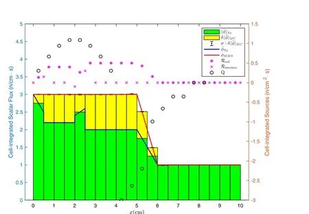
Fig. 9 (Color online) Error estimation for cell-averaged scalar flux using the full SN angular flux

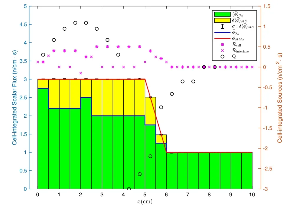
Fig. 10 (Color online) Error estimation for cell-averaged scalar flux using the simplified angular flux

In both Figs. 9 and 10, the cell-interior residual (Rcell)is large when the error is large, and the cell-interface residual (Rinterface) is nonzero only if a discontinuity is present in the SNsolution.It should be pointed out that for simplicity of illustration, we only show the interface residuals on the x+ side, whereas in reality, interface residuals exist on both x+ and x- sides. The forward source (Q)may look unphysical between 4cm and 8cm,as it takes on negative values, which is not unexpected considering that it is a hypothetical source generated from the manufactured solution.

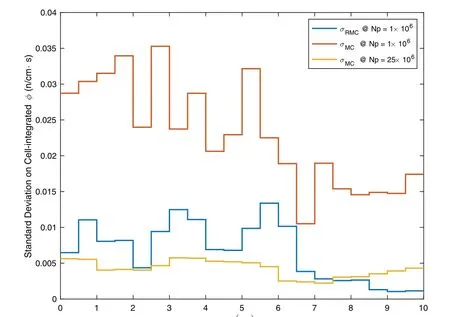
Fig. 11 (Color online) Standard deviations for various calculations

To illustrate the efficiency of the residual Monte Carlo method compared to the standard Monte Carlo method,the standard deviations are analyzed. Figure 11 plots the standard deviation associated with the residual Monte Carlo calculation against those associated with the standard Monte Carlo calculations. From Fig. 11, we can see that when running with 1×106particles, σMC is generally significantly higher than σRMC.If we focus on a particular cell, for example, Cell 5 ([2, 2.5] cm), the difference is about a factor of 5. To match the performance of the residual Monte Carlo calculation in Cell 5, the standard Monte Carlo calculation should be performed with 25 times the number of particles,which translates to 25 times the CPU time.

6.2 Boundary source test

For a more realistic test, we examined the incident flux problem.The problem domain was still[0,10]cm,whereas the background material was set up to mimic graphite,with neutron cross sections Σt ＝4.9435 cm-1and Σs ＝4.9400 cm-1. The isotropic incident neutron angular flux entered through the left boundary, ψ（μ ＞0，x ＝0）＝20 n/cm2s.Vacuum boundary conditions were assumed for the right boundary. There was no distributed source throughout the entire problem domain. The results are presented in Fig. 12.A zoomed-in plot on[0, 2]cm is shown in Fig. 13.

In these plots, φSNis the piecewise linear scalar flux solution given by an S2calculation, 〈φ〉SNis the cell-integrated scalar flux,〈φ〉MC is the same scalar flux computed by the standard Monte Carlo method,and δ〈φ〉RMC is the error computed by the residual Monte Carlo method.It can be seen in these figures,especially in the zoomed-in figure,that the residual Monte Carlo method is capable of estimating the additive error associated with the S2solution.

Fig.12 (Color online)Scalar flux error estimation in graphite with an incoming neutron source

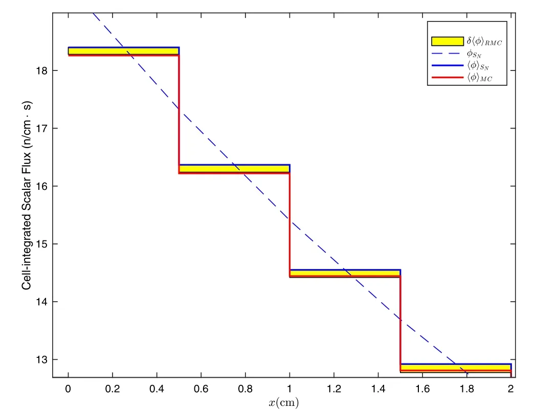
Fig.13 (Color online)Scalar flux error estimation in graphite with an incoming neutron source (zoomed-in)

7 Conclusion and future work

In this paper, we present a nonrecursive residual Monte Carlo method for estimating discretization error associated with the SNtransport calculation. For cases in which the quantity of interest is an angle-space integrated response,we propose a simplified angular flux representation that greatly simplifies the sampling process while still yielding the exact SNerror. We demonstrated the efficacy of our method with a 1-D S4test problem. The results show that our methods are effective at estimating the SNerrors, and for the case of the angle-space integrated response, the simplified method yields exactly the same results as the full SNmethod. Moreover, we propose a modified simplified angular flux representation with double discontinuity,which can be employed to preserve the SNerror in partial currents across cell interfaces.

It should be noted that, although the discussion presented herein is based on LD-FEM spatial discretization,the general methodology can be equally applied to other spatial discretization schemes. In the case of continuous finite element method, which is generally used for the solution of second-order transport equations [20], discontinuities of the angular flux at the cell interfaces disappear,which is the same for the interface residuals.However,the simplified representation is always recommended because of its simplicity when handling residual integral and source sampling. The angular flux discontinuity is inherent to the simplified representation, and we believe that the hassle is worth the benefit.

In future work,we plan to extend the 1-D demonstration to multi-D. The advantage of the residual Monte Carlo method can become more profound as the dimensionality increases.This is partly because the fine-mesh SNcalculation in multi-D is extremely expensive. Full convergence to an SNsolution is unrealistic. Therefore, a viable way of estimating the discretization or iteration error at a fraction of the SNcomputational cost can be valuable.In addition, we would like to integrate the residual Monte Carlo method into a parallel SNsolver framework to determine whether effective parallelization within the existing infrastructure can be achieved.