A lumped mass Chebyshev spectral element method and its application to structural dynamic problems

Wang Jingxiong, Li Hongjing and Xing Haojie

1. Engineering Mechanics Institute, Nanjing Tech University, Nanjing 211816, China

2.Institute of Geophysics, China Earthquake Administration, Beijing 100081, China

Abstract: A diagonal or lumped mass matrix is of great value for time-domain analysis of structural dynamic and wave propagation problems, as the computational efforts can be greatly reduced in the process of mass matrix inversion.In this study, the nodal quadrature method is employed to construct a lumped mass matrix for the Chebyshev spectral element method (CSEM).A Gauss-Lobatto type quadrature, based on Gauss-Lobatto-Chebyshev points with a weighting function of unity, is thus derived.With the aid of this quadrature, the CSEM can take advantage of explicit time-marching schemes and provide an efficient new tool for solving structural dynamic problems.Several types of lumped mass Chebyshev spectral elements are designed, including rod, beam and plate elements.The performance of the developed method is examined via some numerical examples of natural vibration and elastic wave propagation, accompanied by their comparison to that of traditional consistent-mass CSEM or the classical finite element method (FEM).Numerical results indicate that the proposed method displays comparable accuracy as its consistent-mass counterpart, and is more accurate than classical FEM.For the simulation of elastic wave propagation in structures induced by high-frequency loading, this method achieves satisfactory performance in accuracy and efficiency.

Keywords: mass lumping; Chebyshev spectral element method; Gauss-Lobatto-Chebyshev points; Gauss-Lobatto type quadrature; structural dynamic analysis; elastic wave propagation

1 Introduction

The finite element method (FEM) has been an efficient tool for dealing with structural dynamic problems during the past few decades (Satoet al., 2011;Liet al., 2017; Raheemet al., 2018).However, for largescale dynamic problems, e.g., elastic wave propagation in structures induced by high frequency loading, the classical low order FEM (p=1 orp=2) requires fine spatial and temporal discretization to satisfy accuracy and stability requirements (Moseret al., 1999).Therefore, a huge computational cost is generally demanded, which is usually time consuming, even if a high-performance computer system is employed.For this reason, many higher order finite element schemes, such as the p-version finite element method (p-FEM) (Szabó and Babuška, 2011; Issaet al., 1994; Stoykov and Ribeiro,2013), the time domain spectral element method (SEM)(Ostachowiczet al., 2012; Sprague and Geers, 2008),or NURBS-based isogeometric analysis (IGA) (Cottrellet al., 2006; Dedèet al., 2015; Evanset al., 2018) are proposed to reduce the computational burden and supply more accurate solutions.Among these methods, the time domain SEM offers a comparable convergence property and requires substantially less computational cost(Willberget al., 2012; Gervasioet al., 2020).

The time domain SEM, which can be regarded as a high-order FEM, shares the Galerkin principle with FEM, but adopts special element nodes and quadrature rules.It was first proposed by Patera (1984) for solving incompressible Navier-Stokes equations.The SEM is versatile and has been successfully applied in a variety of fields, including, but not limited to seismic wave propagation (Komatitsch and Vilotte, 1998;Komatitsch and Tromp, 1999, 2002a, 2002b; Leeet al., 2008, 2009; Heet al., 2015; Liuet al., 2015, 2018;Yuet al., 2017; Muñoz and Sáez, 2018; Jayalakshmiet al., 2020), structural dynamic analysis (Kudelaet al.,2007a, 2007b; Żak, 2009; Żak and Krawczuk, 2011,2018; Żaket al., 2017; Rekatsinaset al., 2015; Yuet al., 2020), ocean acoustics (Cristini and Komatitsch,2012; Botteroet al., 2016) and geophysical inversion(Tapeet al., 2010; Monteilleret al., 2015).So far, thereare mainly two versions of time domain SEM, namely,the Legendre spectral element method (LSEM) and the Chebyshev spectral element method (CSEM).The LSEM constructs Lagrangian basis functions on Gauss-Lobatto-Legendre (GLL) quadrature points and employs the GLL quadrature rule to evaluate the mass matrix.By means of this operation, which is essentially the nodal quadrature lumping approach, the LSEM obtains lumped mass matrix (LMM) by construction (Komatitsch and Vilotte, 1998; Komatitsch and Tromp, 1999).However,the CSEM constructs Lagrangian basis functions on the Gauss-Lobatto-Chebyshev (GLC) points, but usually uses the Gauss quadrature to evaluate the mass matrix (Dauksher and Emery, 1999, 2000; Żak, 2009).Consequently, the consistent mass matrix (CMM) is derived from the CSEM, which is typically nondiagonal.

Although the early works about SEM started by employing the Chebyshev version, it has not been widely used for various large-scale dynamic problems, since the nondiagonal form mass matrix is computationally inefficient.Several studies have adopted implicit timemarching schemes in CSEM to simulate the propagation of acoustic or seismic waves (Seriani and Priolo, 1994;Seriani, 1997, 1998; Prioloet al., 1994; Priolo, 1999;Zhuet al., 2011).To improve computational efficiency,the mass matrix should be lumped, which enables one to take advantage of the well-established explicit timemarching schemes.Dauksher and Emery (1997, 1999,2000) used the row-sum and diagonal scaling methods to lump the global mass matrix of CSEM for solving scalar wave equations and elastostatic and elastodynamic problems.They proved that solution accuracy is not affected by the mass lumping procedure and the row-sum mass matrix formulation leads to minimal dispersion.Żak (2009) and Żak and Krawczuk (2011)used the row-sum method for mass lumping in the construction of spectral rod and plate elements, based on Chebyshev nodal distribution.Numerical simulations of the wave propagation in rod and plate structures showed that the lumped-mass CSEM is efficient and accurate.Hedayatrasaet al.(2014) accurately modeled the Lamb wave propagation in functionally graded materials by using 2D CSEM with mass matrix lumped by using the row-sum method.Although the row-sum or diagonal scaling techniques pave the way for utilizing explicit algorithms for the CSEM, they lack a solid foundation from a mathematical point of view (Hughes, 1987).Meanwhile, we must bear in mind that before using the row-sum or diagonal scaling methods, the corresponding CMM must first be calculated.This calculation would consume many computational resources because the CMM is fully populated.Apart from these two mass lumping techniques, the nodal quadrature method developed by Fried and Malkus (1975) is mathematically elegant (Zienkiewiczet al., 2013; Cooket al., 1989).It produces LMM by construction without any casual operation.Meanwhile, this approach can retain an order of accuracy as compared to the CMM formulation (Fried and Malkus, 1975; Duczek and Gravenkamp, 2019).

The objective of this study is to propose a lumped mass CSEM, with the aid of nodal quadrature method,to provide an efficient explicit scheme, especially for a dynamic analysis of 1D and 2D structures.This paper is organized as follows.In Section 2, after a brief review of mass lumping procedures, namely, the rowsum, diagonal scaling and nodal quadrature methods,we derived a Gauss-Lobatto type quadrature scheme based on GLC points with the weighting function being unity.By means of this quadrature scheme, a diagonal element mass matrix is automatically constructed for the CSEM.Next, the explicit formulation of this lumped mass CSEM in conjunction with the central difference method is presented.In Section 3, several 1D and 2D lumped mass Chebyshev spectral structural elements are derived, including rod, Timoshenko beam, and Mindlin plate elements.Finally, in Section 4, some examples of the natural vibration and elastic wave propagation in rod, beam and plate structures are investigated to assess the performance of the proposed lumped mass CSEM.

2 Construction of lumped mass CSEM

2.1 Mass lumping techniques

In the standard FEM formulation, the CMM is naturally derived by employing the same set of basic functions for the generation of mass and stiffness matrices.The expression of the element mass matrix is given as:

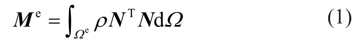
whereΩeis the domain of physical element,ρis mass density, andNis the shape function matrix.The components of the CMM are expressed as:

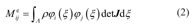
whereΛis the domain of reference element,φi(ξ) is the Lagrange shape function defined on GLC pointξi, and detJis the determinant of the Jacobian matrix.Due to the particularity of GLC points, the Lagrange shape function can be expressed as a truncated expansion of Chebyshev polynomials:

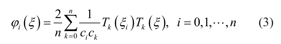
wherenis the element order,Tkis thekth-degree Chebyshev polynomial of the first kind, and is given as:

The coefficientciis defined as:

As we know, in the context of FEM, a lumped mass matrix is preferable for dynamic analysis with explicit time-marching schemes.The procedure for making the mass matrix diagonal is known as “mass lumping”.This section provides a brief review of the three most frequently used mass lumping schemes.

(1) Row-sum method

In the row-sum method, the entries on each row of the CMM are accumulated according to the main diagonal term.This method is easy to implement, but it may lead to zero or negative mass for some elements (e.g.,the 6-node quadratic triangular element and the 8-node serendipity quadrilateral element—see Zienkiewiczet al., 2013), which is undesirable for dynamic analysis.This lumping method can be expressed as:

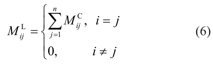
whereandare the components of LMM and CMM, respectively.

(2) Diagonal scaling method

The diagonal scaling method, which also is referred to as “HRZ lumping” (Cooket al., 1989), was proposed by Hintonet al.(1976).In this method, the diagonal terms of the CMM are scaled and off-diagonal terms are set to be zero, with total mass being preserved.This method can always generate positive diagonal masses,but it lacks a mathematical foundation (Hughes, 1987).The expression of this method is as follows:

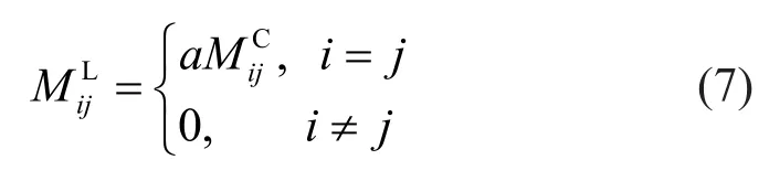
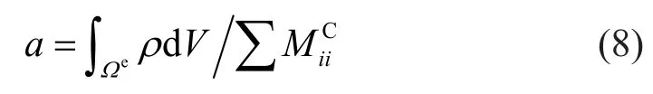
The scaling coefficientais the ratio of the total mass of the element to the sum of the diagonal terms of CMM:

(3) Nodal quadrature method

The nodal quadrature method is mathematically appealing, since only the quadrature scheme must be changed and no extra work is required.It uses element nodes as the quadrature points for the evaluation of mass matrix.In other words, the interpolation points where Lagrange shape functions are defined would be placed to be completely coincident with quadrature points.Usually,the Gauss-Lobatto quadrature scheme is adopted, which is like the Gauss-Legendre quadrature rule, except that the end points of the interval are included.Using this quadrature scheme, the mass matrix integral of an-th order element is computed as:

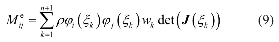
whereξkare the coordinates of the Gauss-Lobatto quadrature points over the standard interval [-1,1] andwkis the quadrature weight.

As we know, the Lagrange polynomials possess the Kronecker delta property, which means each shape function is equal to one at its defining node and zero at all other nodes.Therefore, when using the Gauss-Lobatto quadrature to evaluate the element mass matrix,the components in which two Lagrange polynomials are multiplied, as shown in Eq.(9), would be nonzero at diagonal terms and zero at all off-diagonal terms.Thus,an LMM is automatically obtained through the nodal quadrature method, without any additional operation,which is a more straightforward approach than that of the row-sum and diagonal scaling methods.

According to the above, to construct a lumped mass CSEM using the nodal quadrature method, a Gauss-Lobatto type quadrature rule based on GLC points (the element nodes) should be employed to evaluate the mass matrix.Although the CSEM is constructed based on the GLC quadrature points, the GLC quadrature rule(Davis and Rabinowitz, 1984) itself is not appropriate for the evaluation of the mass matrix of CSEM.That is because the GLC quadrature has a weighting function, while for the mass matrix of CSEM, the integrand is the product of two Lagrange polynomials and the weighting function equals unity, as shown in Eq.(2).Therefore, employing a Gauss-Lobatto type quadrature rule through the GLC points, but with weighting function unity, would be a better choice.Such a quadrature scheme is described in the next section.

2.2 The Gauss-Lobatto quadrature based on GLC points

In this section, we derive a Gauss-Lobatto type quadrature scheme through the GLC points with weighting function equal to unity, according to the general form of the Gaussian quadrature.First, we approximate the integrandf(ξ) with a series of Lagrange interpolation polynomials,

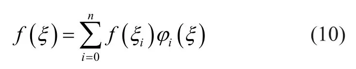
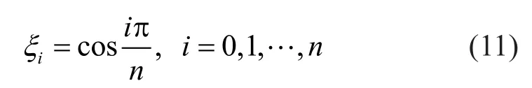
whereξiis the GLC point whose explicit expression can be written as:

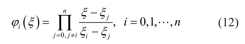
φi(ξ) is the Lagrange interpolant defined atξi

Then, the definite integration off(ξ) over the interval[-1,1] can be approximated as

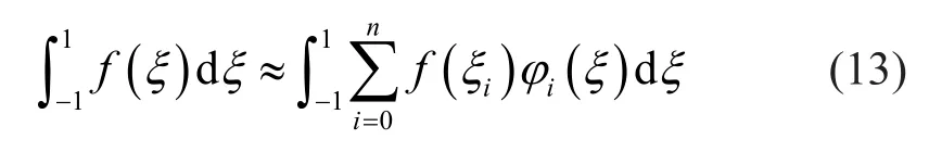
Interchanging the integral and summation produces

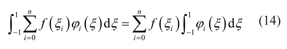
By defining the integration of the Lagrange interpolant as the quadrature weight, this quadrature rule could be rewritten as the following compact form:

where the quadrature weight is

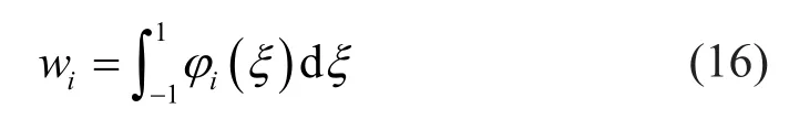
Table 1 shows the weights and abscissas of the derived quadrature formula for the first 5 degrees.

As we know, the (n+1)-point interpolatory quadrature formula has at least ann-order of accuracy.If the quadrature formula withn+1 points cannot exactly integrate a polynomial of the degreen+1, then the order of accuracy of this quadrature formula is equal ton.For example, the accurate result for the integration ofx4over the reference domain [-1,1] is 0.4; but if we use the quadrature derived in this section with 4 points,the quadrature result would be 0.3333.That is, this quadrature formula withn+1 points cannot precisely integrate the polynomial of degreen+1.Thus, the order of accuracy of this quadrature rule isn.

A simplified numerical test is conducted here to examine the performance of the derived quadrature for evaluating mass matrix.Considering anth-order element, the shape function is a polynomial of degreen, and the integrand of mass matrix is a polynomial of degree 2n.To generate a lumped mass matrix,the number of quadrature points should ben+1.For simplicity, we suppose the integrand will be a simple polynomialx2n.Table 2 shows the results of the derived quadrature for evaluatingx2nover the reference domain withn+1 points.The quadrature error with respect to an analytical solution decreases rapidly with an increase in polynomial degree.For example, the quadrature error forx12, which corresponds to the 6th-order element, is less than 4%.Therefore, one can expect the error induced by this quadrature to become trivial if the element order is sufficiently high.

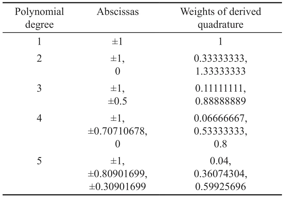
Table 1 Weights of the Gauss-Lobatto quadrature based on GLC points

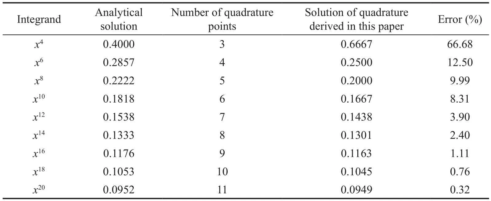
Table 2 Error of the derived quadrature for integrating x2n with n+1 points

2.3 Equivalence between the nodal quadrature and row-sum methods

As demonstrated by Duczek and Gravenkamp(2019), if mass density and the element metric are constant, the row-sum and the nodal quadrature methodare equivalent for the LSEM.In this section, we prove that for the CSEM the nodal quadrature mass lumping technique also is equivalent to the row-sum method under certain conditions.For clarity, we provide a demonstration for the 1-D case here; its conclusion can easily be extended to 2-D and 3-D cases due to their tensor product formulation.

At first, we assume that mass density and the Jacobian are constants within the element.Using the quadrature rule derived and reported on in Section 2.2, the diagonal terms of the mass matrix of the CSEM are evaluated as:

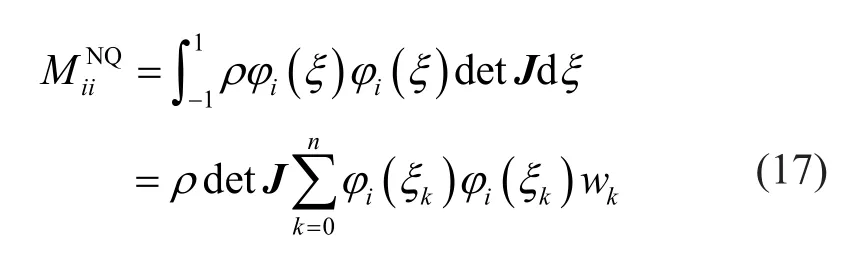
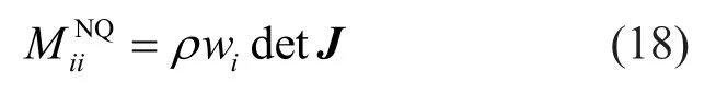
where the superscript “NQ” denotes the nodal quadrature method.Considering the Kronecker delta property of the Lagrange shape function, Eq.(17) can be simplified as

For the row-sum method, the diagonal term of the mass matrix would be

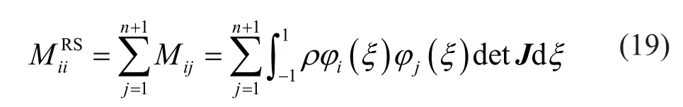
where the superscript “RS” denotes the row-sum method.Interchanging the integral and summation yields

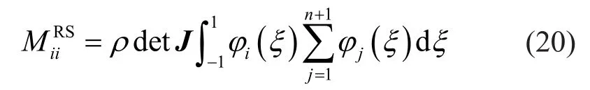
Since the Lagrange interpolants on the interval[-1,1] form a partition of unity, Eq.(20) can be further expressed as

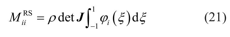
Recalling the quadrature weight defined in Eq.(16),it is obvious that Eq.(18) and Eq.(21) are identical.In other words, the nodal quadrature method leads to the same lumped mass matrix as the row-sum method for the CSEM.It is worth noting that although the resulting lumped mass matrices are identical, the nodal quadrature method is more straightforward and efficient than the row-sum method.

2.4 Lumped mass CSEM formulation for structural dynamic problems

The formulation of the time domain CSEM for structural dynamic problems is analogous to that of classical FEM.The crucial differences between them are the nodal locations and the quadrature rule for evaluating element characteristic matrices.As previously mentioned, the local node coordinates of the Chebyshev spectral element (CSE) are the GLC points, as expressed by Eq.(11).Lagrange interpolating polynomials through the GLC points are constructed as element shape functions, as provided in Eq.(12).Following the classical FEM procedures, we finally obtain the wellknown semi-discrete equations

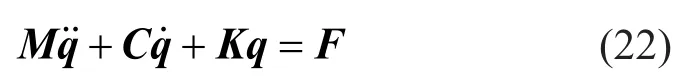
whereMis the global mass matrix,Cis the global damping matrix,Kis the global stiffness matrix,Fis the vector of time-dependent nodal forces, andqis the nodal displacement vector.In the present paper,we evaluate the element mass matrix using the Gauss-Lobatto type quadrature derived and listed in Section 2.2.For example, the element mass matrix of 1-D CSE is computed as

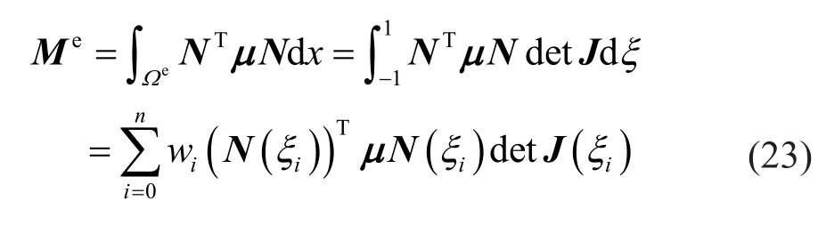
whereμis the mass density matrix.The element stiffness matrix can be evaluated by using the exact Gauss-Legendre quadrature

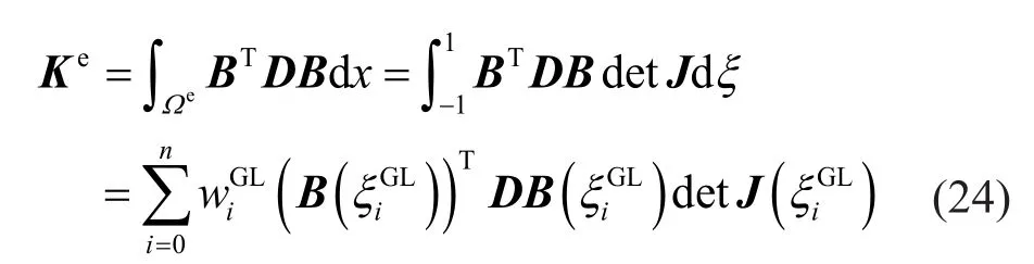
whereBdenotes the strain-displacement matrix,Ddenotes the elasticity matrix, andandare the abscissas and weights of the Gauss-Legendre quadrature,respectively.

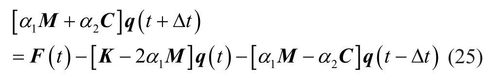
To construct a full explicit scheme for a largescale structural dynamic problem, we use the central difference method to conduct time integration.Thus, the displacement vector at timet+Δtcan be obtained as

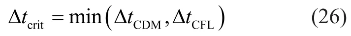
where ΔtCDMis the critical time step, determined by the maximum eigenvalue (Belytschkoet al., 2013)

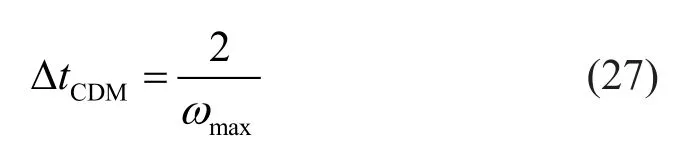
whereωmaxis the maximum frequency of the system.ΔtCFLis the critical time step, determined by the Courant-Friedrichs-Lewy (CFL) condition

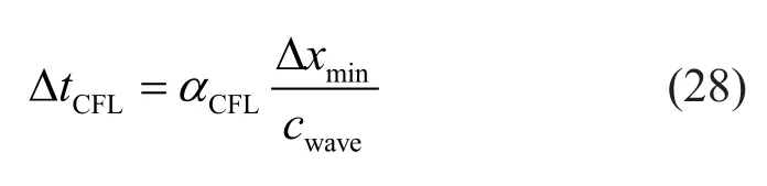
where Δxminis smallest distance between any two nodes in the mesh,αCFLis the dimensionless CFL number, andcwaveis the theoretical elastic wave speed.

In this paper, the damping effect of the structure is not considered, viz.C=0.Since the element mass matrix is diagonal by construction, the assembled global mass matrix can be stored as a vector that contains only diagonal terms.In addition, the element-by-element(EBE) technique (Zhanget al., 2021) is used here to avoid storage and calculation of a large sparse global stiffness matrix.Hence, the displacement vector at each time step is obtained by solving the following equation:

where

In this way, Eq.(25) reduces toNuncoupled algebraic equations, which requires a much lesser storage requirement and computational burden.

3 Structural element formulations

This section presents the formulations of several lumped mass Chebyshev spectral structural elements by using the Gauss-Lobatto type quadrature, which was derived and reported on in Section 2.2, for evaluating element mass matrix.All these elements are built in isoparametric form.First, 1-D structural elements,including a rod element and a Timoshenko beam element, are presented.Next, 2-D Mindlin plate element is established based on the tensor product formulation.

3.1 Rod element

The rod element has only one degree of freedom per node, i.e., the axial displacement.For an isotropic rod,the mass density matrix is

whereρis the mass density andAis the cross-sectional area.The strain-displacement matrix is given as

and the elasticity matrixDis

whereEis Young′s modulus.

3.2 Timoshenko beam element

For the Timoshenko beam element, there are two degrees of freedom per node, namely, the deflectionwand the rotation of cross-sectionθ.Axial displacement is not considered herein.We interpolatewandθseparately with the same set of Lagrange shape functions.Hence,the displacement field can be expressed as

where the element shape function matrix is given by

and the nodal displacement vector is

Based on the Timoshenko beam theory, the mass density matrix is described by

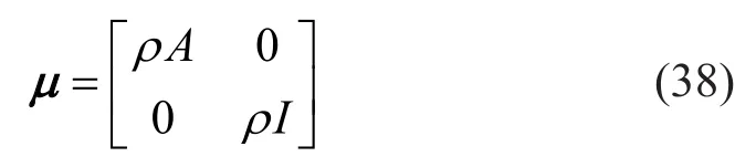
whereIis the moment of inertia.The element stiffness matrix can be divided into a bending part and a shear part, viz.

For the bending stiffness matrix, the elasticity matrix is

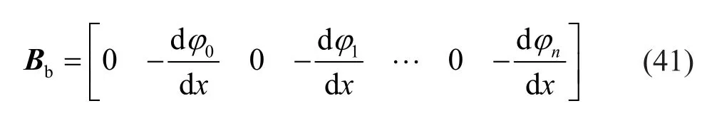
And the strain-displacement matrixBbis written as

For the shear stiffness matrix, the elasticity matrix is

withGbeing the shear modulus,vthePoisson′s ratio,andκthe shear correction factor.The strain-displacement matrixBsis given by

3.3 Mindlin plate element

According to Mindlin plate theory, there are three independent degrees of freedom per node, namely, the deflectionw, rotationθxandθy.The number of element nodes is written asng=(n+1)2forn-th order element.The element displacement field can be expressed as

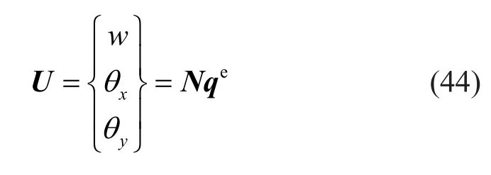
where the element shape function matrix is given by

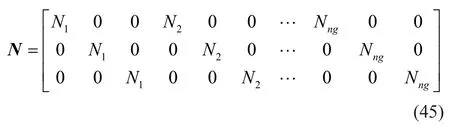
and the nodal displacement vector is

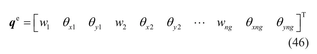
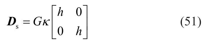
For the Mindlin plate element, the mass density matrix is

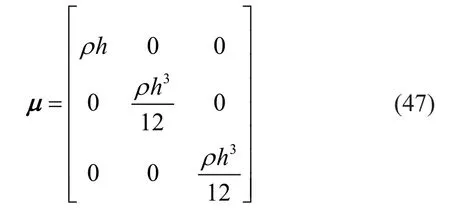
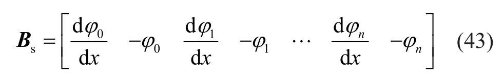
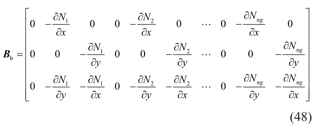
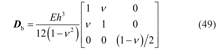
wherehis the thickness of the plate.The stiffness matrix of Mindlin plate element consists of a bending part and a shear part.The strain-displacement matrix for the bending stiffness matrix is written as:

and the elasticity matrix is

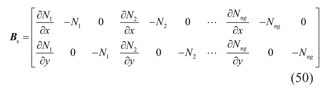
For the shear stiffness matrix, the strain-displacement matrix is given by:

and the elasticity matrix is

4 Numerical results

In this section, we verify the validity of the newly proposed lumped-mass CSEM for solving 1D and 2D structural dynamic problems.First, the natural frequencies of rod, beam and plate are examined as a benchmark test.A comparison study is made among the proposed Chebyshev spectral element method with lumped mass matrix (CSEM-LMM), the conventional Chebyshev spectral element method with consistent mass matrix (CSEM-CMM), and the classical FEM.It is noted that for the CSEM-LMM, the mass matrix is evaluated utilizing the Gauss-Lobatto type quadrature derived and described in Section 2.2.For the CSEM-CMM, the mass matrix is evaluated by employing the standard Gauss quadrature.Next, elastic wave propagation in rod, beam and plate are investigated to assess the performance of the proposed method for high-frequency problems.

4.1 Natural frequency of a cantilever rod

In this paper, we use the root-mean-square error to evaluate the accuracy of numerical results of natural vibration frequencies

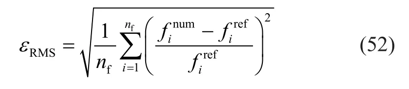
wherenfis the number of frequencies; the superscript“num” indicates the results obtained from numerical methods, namely, the CSEM-LMM, CSEM-CMM and FEM; the superscript “ref” denotes reference solutions—i.e., exact solutions computed according to existing structural dynamics or vibration theories.

The natural vibration of a cantilever rod is studied by first using the rod elements derived in Section 3.1.As illustrated in Fig.1, this rod is fixed at the left end and is free at right end.The geometric and material parameters of the rod are as follows: lengthL=3 m, cross-sectional widthb=0.02 m, heighth=0.1 m, mass densityρ=7800 kg/m3,and Young′s modulusE=210 GPa.For both CSEMLMM and CSEM-CMM, the model is discretized by including three types of regular grids, denoted as mesh A, mesh B and mesh C, respectively.Mesh A consists of three identical spectral elements in a size of Δx=1 m;mesh B has six elements in a size of Δx=0.5 m, and mesh C has 10 elements in a size of Δx=0.3 m.Table 3 lists the values of first six natural frequencies computed by using different meshes, where the element orderpkeeps four.For the free axial vibration of a cantilever rod, the analytical solution for theith frequency is provided by Craig and Kurdila (2006):

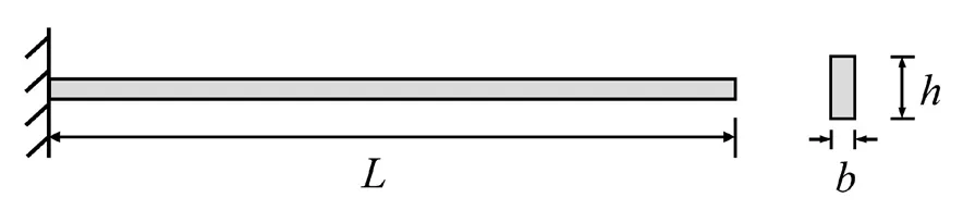
Fig.1 Illustration of the cantilever rod

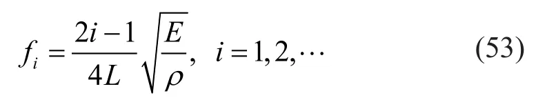
The results obtained by Eq.(53) are listed in the last column of Table 3 as reference solutions to check the accuracy of numerical results.As shown in Table 3,the results from two different kinds of CSEMs are all in good agreement with the reference solutions.As the mesh becomes denser, the numerical results gradually become closer to the exact values.

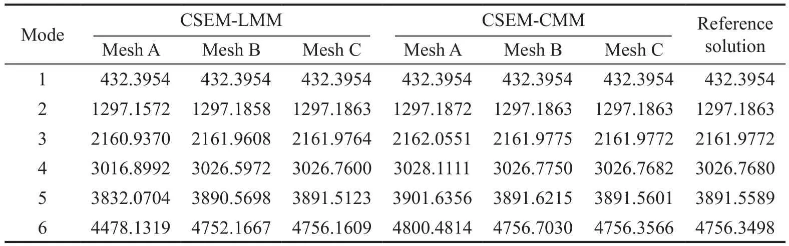
Table 3 The first six natural frequencies (Hz) of a cantilever rod (p=4)

Figure 2 plots the variation of the root-mean-square error of the first six eigenvalues with respect to the number of degrees of freedom (ndof).Two different mesh refinement methods are applied to both the CSEMLMM and CSEM-CMM, namelyp-refinement andh-refinement.Forp-refinement, the element size keeps Δx=1 m (three elements in the model) and the element order increases from 4 to 24.Forh-refinement, the element order remainsp=4 and the number of elements rises from 3 to 18.Besides, the results of classical FEM obtained from the commercial software ABAQUS also are plotted for comparison.The two-node linear truss/rod element T2D2 in ABAQUS is adopted for the analysis, andh-refinement is performed on the FEM mesh.It can be seen from Fig.2 that bothp-refinement andh-refinement can lead to a gradual decrease in error.However, for both CSEM-LMM and CSEM-CMM, thep-refinement exhibits a more rapid convergence than theh-refinement.Whenp-refinement is conducted, the error curve of CSEM-LMM is very close to that of CSEMCMM.Whenh-refinement is used, the accuracy ofCSEM-LMM is slightly inferior to that of the CSEMCMM, but it is still much better than the conventional FEM solutions.

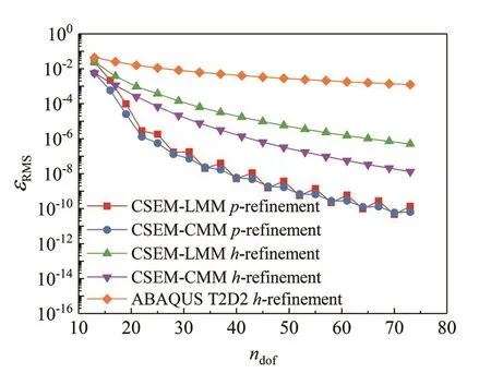
Fig.2 Root-mean-square error of the first six natural frequencies for the cantilever rod

4.2 Natural vibration of a simply supported Timoshenko beam

The natural vibration of a simply supported Timoshenko beam is another 1-D benchmark problem.The beam is sketched in Fig.3.The geometric parameters of the beam are taken as lengthL=3 m, cross-sectional widthb=0.02 m, and heighth=0.1 m.The material parameters are mass densityρ=7800 kg/m3, Poisson′s ratiov=0.3 and Young′s modulusE=210 GPa.According to the Timoshenko beam theory, the analytical solution for the free transverse vibration frequencies of the beam is determined by the following equation (Rao, 2018)

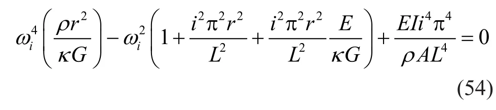
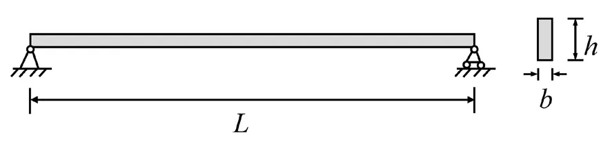
Fig.3 Illustration of the simply supported beam

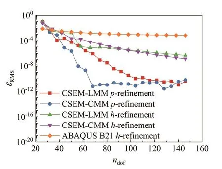
Fig.4 Root-mean-square error of the first six natural frequencies for the beam

Herein, the beam is discretized with three normalized meshes.Mesh A refers to element size Δx=1 m, for a total of three elements; Mesh B refers to Δx=0.5 m, for a total of six elements; Mesh C refers to Δx=0.3 m, for a total of 10 elements.Table 4 shows the first six natural frequencies of different models, with the element orderp=4.The reference results calculated according to Eq.(54)are listed in the last column.It is shown that the two forms of CSEM can achieve good results for this problem.The numerical results approach those of the analytical solution as the mesh become denser.Figure 4 depicts the root-mean-square error of the first six natural frequencies for the simply supported beam.The samep-refinement andh-refinement procedures, as described in Section 4.1, are adopted here for the Timoshenko beam.Meanwhile, classical FEM solutions from ABAQUS are plotted in the same figure.The 2-node linear beam element B21, which also is based on Timoshenko beam theory, is employed for the FEM simulation.As can be observed, in most cases the errors of both CSEM-LMM and CSEM-CMM are much smaller than those of the ABAQUS solutions.For this eigenvalue problem, the two different CSEMs can achieve similar convergence underh-refinement.The CSEM-LMM sometimes provides better accuracy than does the CSEM-CMM.Whenp-refinement is conducted, the CSEM-LMM converges steadily, but the CSEM-CMM has an error plateau.As stated by Duczek and Gravenkamp (2019),this behavior is attributed to the fact that numerical errors independent of the discretization dominate the overall convergence.

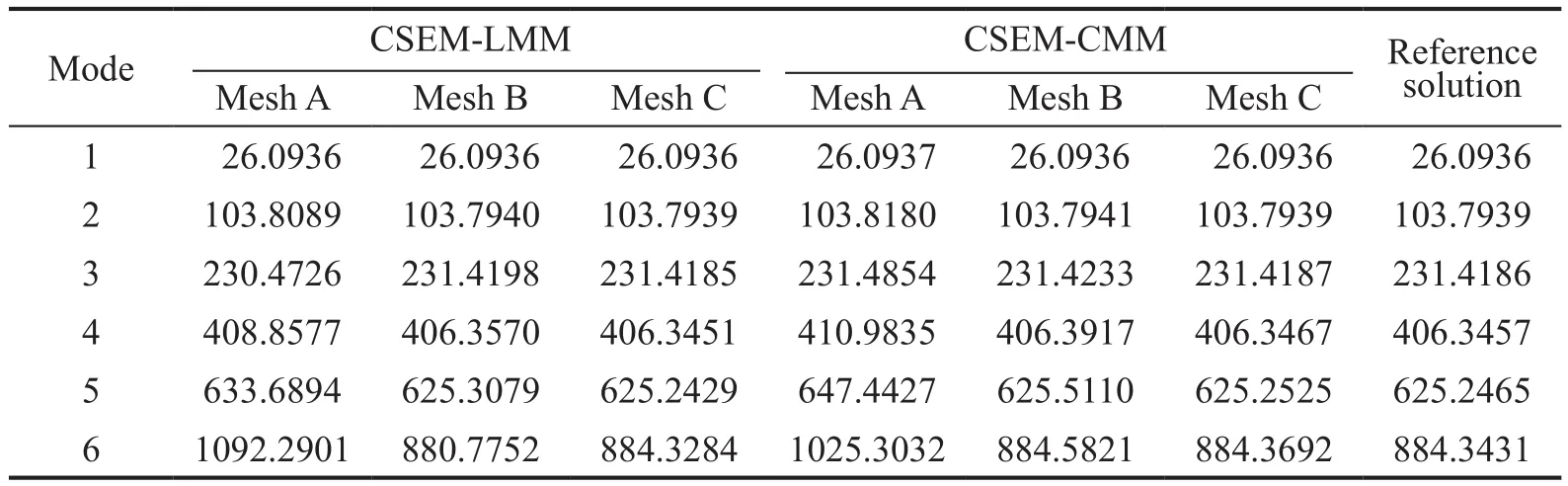
Table 4 The first six natural frequencies (Hz) of the simply supported beam (p=4)

4.3 Natural vibration of a four-edges simply supported rectangular plate

In this section we present an eigenvalue analysis for a rectangular plate that is simply supported on four edges,as sketched in Fig.5.The Mindlin plate element derived and reported on in Section 3.3 is employed to discretize the model.The geometry of the plate is the length in thexdirectionLa=3 m, the width in theydirectionLb=3 m,and a thicknessh=0.003 m.The material parameters are the same as that of the Timoshenko beam, as described in Section 4.2.

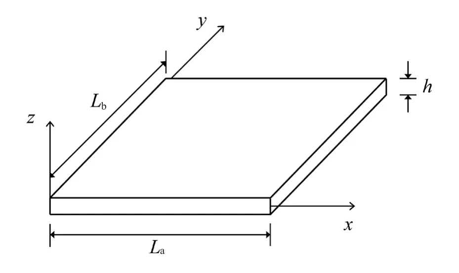
Fig.5 Illustration of the rectangular Mindlin plate

The analytical solution based on Kirchhoff platetheory and the approximate solution based on Mindlin plate theory are employed as references.According to the Kirchhoff theory, the natural frequencies of a rectangular plate with four edges simply supported is (Rao, 2007)

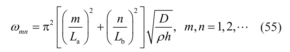
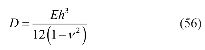
wheremandndenote the number of half sine waves inxandydirections, respectively, andDis the flexural rigidity of the plate:

Based on the Mindlin plate theory, the natural frequencies of a four-edges simply supported rectangular plate is given by Liewet al.(1998)

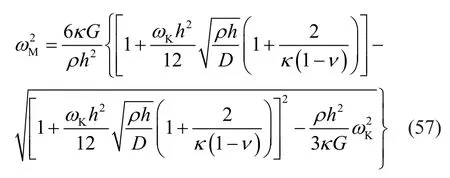
whereωMdenotes the Mindlin solution andωKrepresents the Kirchhoff solution, as taken from Eq.(55).

Table 5 shows the first nine natural frequencies of the four-edges simply supported plate.The Kirchhoffand Mindlin solutions are listed in the last two columns for reference.Since the plate is very thin (h/La=10-3), the Mindlin solution is only slightly lower than that of the Kirchhoff solution.Here, three different regular grids are deployed, with the element order keeping four.Mesh A employs a single element to execute the modeling, i.e.,Δx=Δy=3 m; Mesh B represents Δx=Δy=1.5 m, for a total of four spectral elements; Mesh C represents Δx=Δy=1 m,for a total of nine spectral elements.It can be seen that the two CSEMs can provide reasonable eigenvalues even on very coarse meshes.

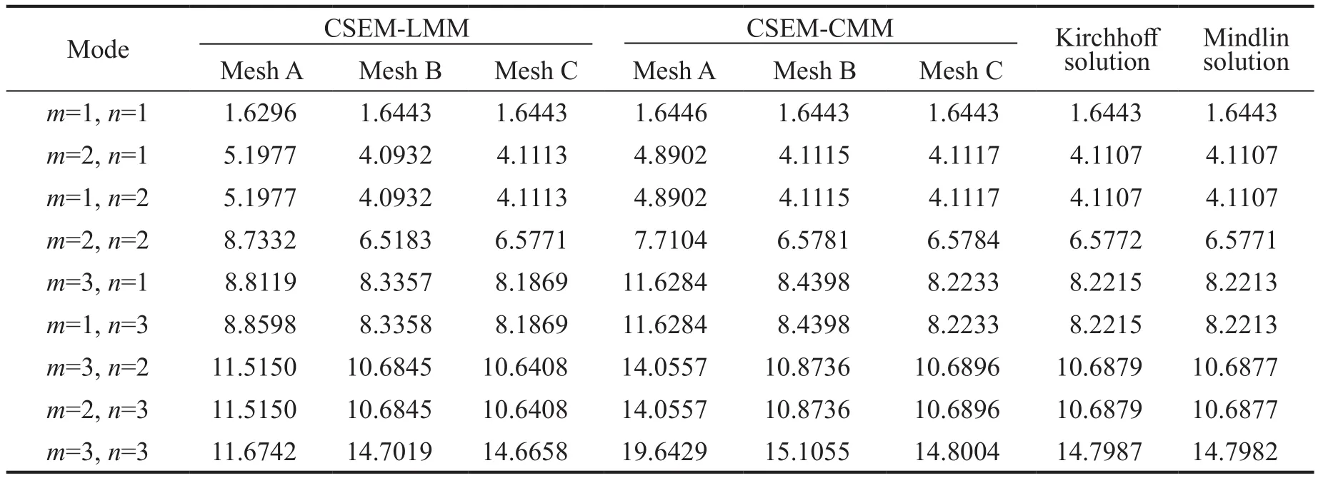
Table 5 The first nine natural frequencies (Hz) of a four-edges simply supported plate (p=4)

Figure 6 depicts the root-mean-square error of the first nine natural frequencies with respect to element order, where the plate is simulated by only one element.Since the plate is thin enough, the error is calculated with respect to the Kirchhoff solution.As shown in Fig.6, the curves of these two methods show goodconvergence with the increment of element order.For both CSEM-LMM and CSEM-CMM, a single element with order greater than seven can reduce the error to less than 1%.Although sometimes the error of CSEM-LMM is larger than that of CSEM-CMM, it is rather small, and sufficiently exact from an engineering point of view.Besides, when the element order is high enough (p=11),the errors produced by CSEM-LMM and CSEM-CMM are not obviously different.

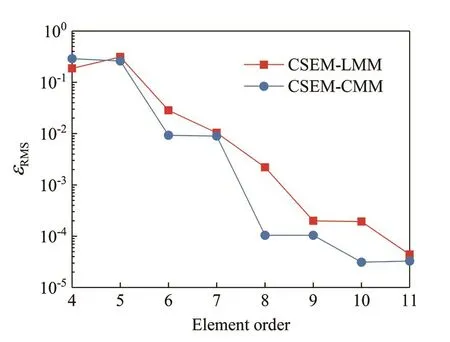
Fig.6 The root-mean-square error of the first nine natural frequencies for the four-edges simply supported plate under p-refinement

Figure 7 plots the root-mean-square error of the first nine natural frequencies with respect to the number of nodes (nnode) in the model.Meanwhile, the FEM results obtained by using ABAQUS with the 4-node generalpurpose shell element S4 also is plotted.For these three methods, the number of elements per side increases gradually, and the element order remains constant (p=4 for CSEM-LMM and CSEM-CMM,p=1 for ABAQUS S4).As illustrated in Fig.7, the two different CSEM formulations lead to a much faster convergence than does the conventional FEM.The results produced by CSEM-LMM are occasionally more accurate than those obtained by CSEM-CMM.

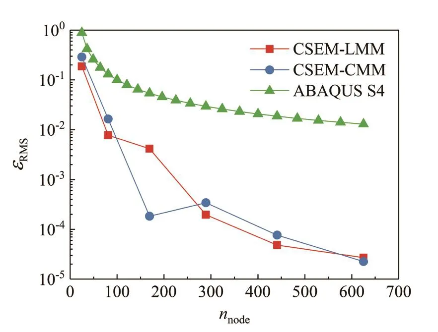
Fig.7 The root-mean-square error of the first nine natural frequencies for the four-edges simply supported plate under h-refinement

4.4 Wave propagation in a rod with additional mass

This section investigates elastic wave propagation in an aluminum rod with additional mass.For purposes of comparison, the example is the same as that explored by Kudelaet al.(2007a) using the LSEM, as well as Wanget al.(2010) who used the discrete singular convolution(DSC).As shown in Fig.8, the rod is free at both ends and an additional mass is situated in the middle.The rod has a length ofL=2 m and a rectangular cross-section with a width ofb=0.01 m, and a height ofh=0.001 m.Material properties include mass densityρ=2700 kg/m3and Young′s modulusE=70 GPa.

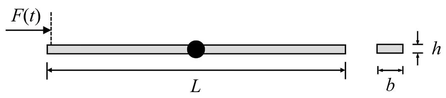
Fig.8 Illustration of a rod with additional mass

The rod is subjected to a time-dependent force at about 0.01 m away from the left end of the rod.The excitation signal is a 5-cycle sine pulse modulated by a Hann window.The carrier frequency is chosen as 100 kHz.Thus, the modulation frequency is 20 kHz for the 5-cycle signal.Figure 9 depicts the excitation signal in time and frequency domains.

First, a convergence study is conducted on the rod without additional mass.Figure 10 plots the relative error between simulated and theoretical wave speeds.Note that for the longitudinal wave in the rod, the theoretical wave speed is.Figure 10 shows the simulated results approach to the analytical solution,with an increment of the number of degrees of freedom or the element order.For example, when the rod is discretized by 80 eight-node rod elements (ndof=561),the relative error is less than 3%.Figure 11 shows the snapshots of wave propagation in the rod using this discretization.The location of the theoretical wave front is represented by the dashed line as it appears in Fig.11.As can be observed, the simulated wave speed agrees well with the theoretical group speed.

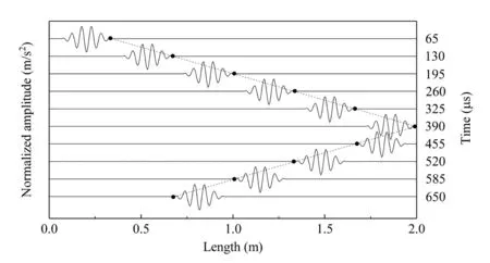
Fig.11 Snapshots of elastic wave propagation in rod without additional mass

Figure 12, in which 80 eight-node elements also are listed, illustrates the acceleration response history recorded at the left end, with additional mass equal to4% of total mass.For clarity, the abscissa is in distance,which is the product of time and the wave speed.The first visible peak denotes the excitation signal.The second and third peak represent the reflected wave from the additional mass and the free end of the rod, respectively.As can be observed, the second peak occurs at a distance of 2 m.That is to say, the excitation is reflected from a distance of 1 m, which is exactly the center of the rod.Therefore, the location of the additional mass is accurately detected.This simulation result also is in good agreement with the numerical results obtained by Kudelaet al.(2007a) and Wanget al.(2010).

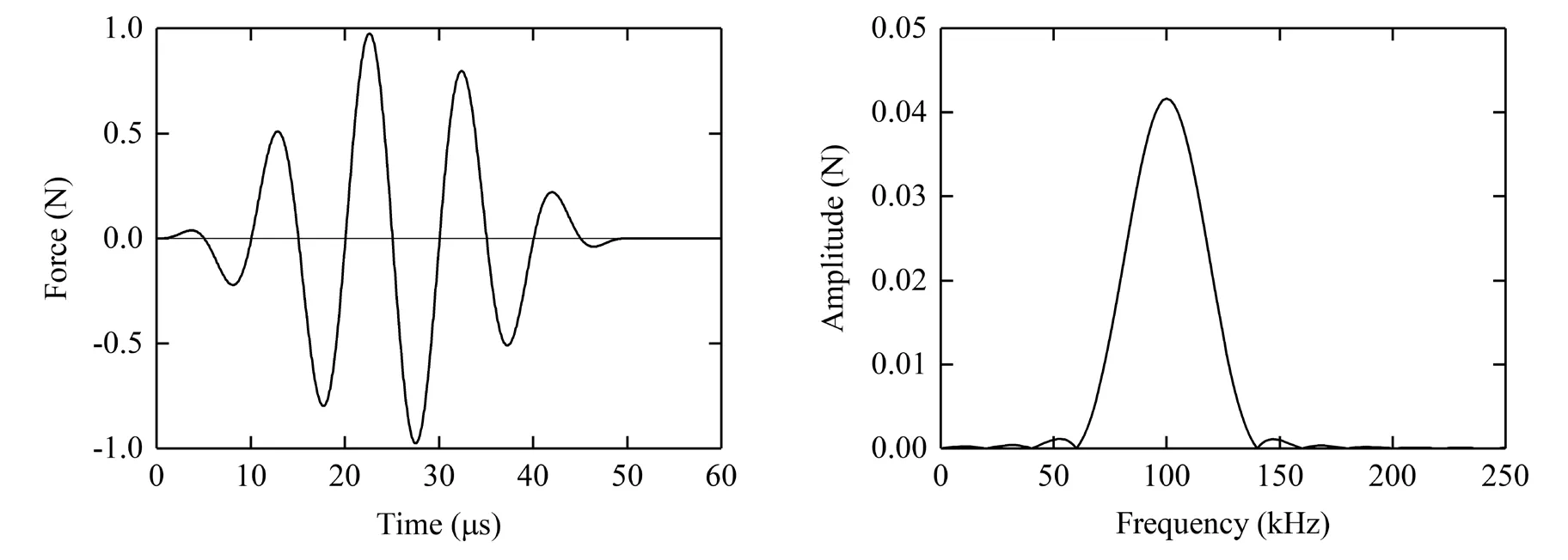
Fig.9 Excitation signal in time and frequency domains

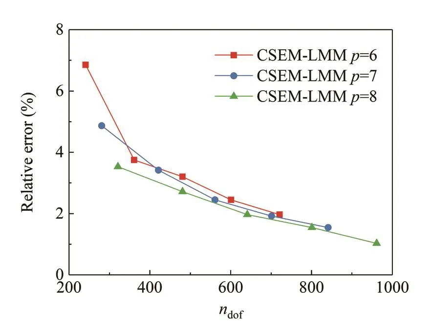
Fig.10 Relative error between simulated and theoretical wave speeds in the rod

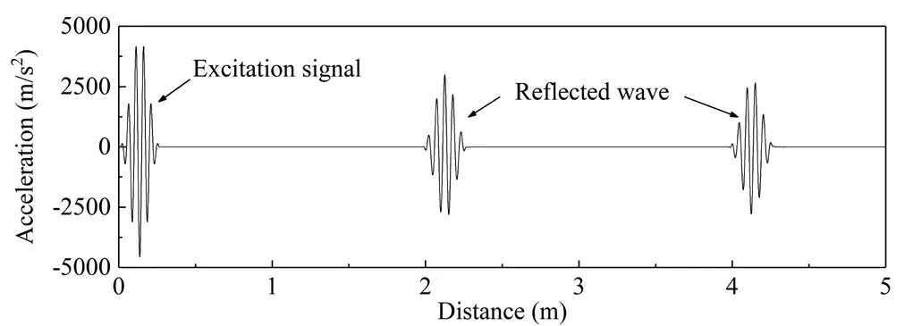
Fig.12 Response history recorded at the left end of the rod with 4% additional mass

Figure 13 plots the snapshots of wave propagation at the timet=294.6 μs to show the effect of additional mass on the waveform.The backward wave corresponds to the wave reflected by the additional mass, and the forward wave is the wave pass through additional mass.As can be seen from Fig.13, the backward wave is not affected by the value of additional mass.However, the amplitude of forward wave obviously decreases with an increase in additional mass.

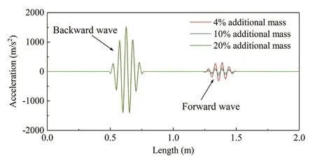
Fig.13 Waveforms of the rod with varying additional mass at time t=294.6 μs

4.5 Wave propagation in a Timoshenko beam

In this section, the flexural elastic wave propagation in a Timoshenko beam is investigated.For comparison,the beam model is identical to that analyzed by Kudelaet al.(2007a), with time domain LSEM.As shown in Fig.14, a time-dependent force is applied at the locationd=1 cm from the left end.The excitation signal and the material parameters are the same as those for the rod referred to in the previous section.The dimensions of the beam areL=3 m, a width ofb=0.06 m, and a height ofh=0.06 m.In this case, the cut-off frequency of the second mode can be analytically calculated asfcut=26.19 kHz(Doyle, 1989).Since the excitation frequency is beyond the cut-off frequency, the second mode wave should be separated in the response of the beam.

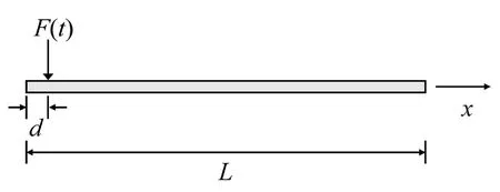
Fig.14 A Timoshenko beam subjected to an excitation signal

Figure 15 shows the relative error between the simulated and theoretical wave speeds of the first mode.The theoretical wave speed of first mode for the Timoshenko beam analyzed here is(Doyle, 1989).As can be seen, bothp-refinement andh-refinement can lead to a convergence of the simulated wave speed.Generally,thep-refinement approach is more efficient than theh-refinement technique.For example, when the element order is 8, only 80 elements (ndof=1282) are needed to reduce the error to less than 4%.

Figure 16 illustrates the snapshots of the elastic wave propagating in the beam.Herein, the beam is divided intoone hundred 8-node Chebyshev spectral beam elements,as derived and described in Section 3.2.It is the same mesh scheme as that adopted by Kudelaet al.(2007a).As can be observed, the second mode wave is captured in the simulation.Its amplitude is much smaller than that of the first mode wave, but it travels with a faster wave speed.The theoretical wave front of first mode is plotted by the dashed line shown in Fig.16.The response signal always travels with proper wave speed.However,in Kudelaet al.(2007a), the first wave simulated by LSEM travels much faster than the theoretical speed.This example indicates that the proposed lumped mass CSEM is capable of simulating elastic wave propagation in beams, and in some cases may behave better than the LSEM.

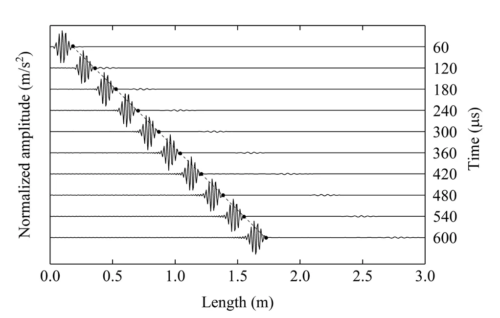
Fig.16 Snapshots of elastic wave propagation in a beam

4.6 Wave propagation in a rectangular plate

This section presents modeling of the Lamb wave propagation in an aluminum plate.The Mindlin plate element derived in Section 3.3 is used to discretize the model.Due to the formulation based on Mindlin plate theory, only the anti-symmetric mode can be simulated.The dimension of the plate isLa=Lb=1 m with a thickness ofh=0.01 m.The material parameters include mass densityρ=2700 kg/m3, Young′s modulusE=70 GPa, and Poisson′s ratiov=0.33.The 5-cycle sine pulse described in Section 4.4 is applied at the center of the plate, which is denoted as point A in Fig.17.Since the frequency of the excitation signal is lower than the cut-off frequency(141.6 kHz) of the first anti-symmetric mode, only theA0mode would be excited in the plate.

Fig.15 Relative error between simulated and theoretical wave speeds in the beam

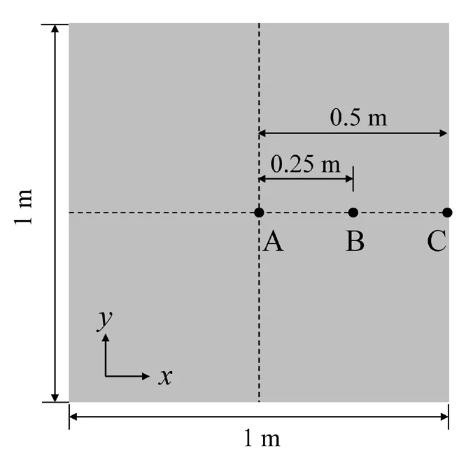
Fig.17 Illustration of the aluminum plate

Figure 18 shows the relative error between simulated and theoretical group speeds.The theoretical group speed is determined by use of the Rayleigh-Lamb equations (Rose, 2014).As can be seen from Fig.18,the error decreases with an increase in the number of degrees of freedom and the element order.High order elements can provide good accuracy even on a coarse mesh, e.g., 30×30 7th-order elements (ndof=133563) lead to an error of less than 5%.

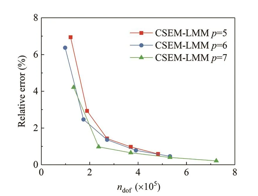
Fig.18 Relative error between simulated and theoretical wave speeds in the plate

Figure 19 depicts the response histories of three different observing points on the plate, which are modeled by the use of 50×50 49-node Mindlin plate elements.The curve of point A represents the excitation signal.The amplitudes of the response of point B and point C are substantially smaller than that of the excitation signal due to energy diffusion during wave propagation.The wave reflected from the free boundary is visible in the curve of point B.Figure 20 presents a series of snapshots at different time instances to show the process of elastic wave propagation.It can be seen from Fig.20that a pure anti-symmetric mode is correctly excited.The Lamb wave in different directions propagates with the same group speed.The waves reflected from the free boundaries are visible in Fig.20.

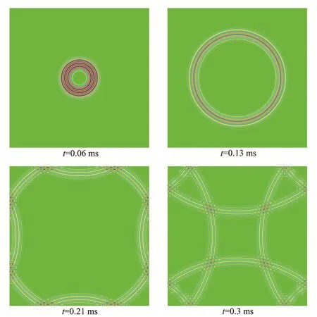
Fig.20 Snapshots of the A0 mode Lamb wave in the aluminum plate

5 Conclusions

This paper is devoted to developing a lumped mass Chebyshev spectral element method for solving structural dynamic problems.A brief review of mass lumping techniques reveals the advantages of the nodal quadrature method, from mathematical and computational perspectives.To employ the nodal quadrature method for mass lumping in CSEM, it is deduced that the Gauss-Lobatto-type quadrature, based on the Gauss-Lobatto-Chebyshev points with weighting function equal to unity.With the aid of this quadrature scheme, a lumped mass CSEM is constructed with a solid mathematical foundation.Meanwhile, it enables us to implement explicit time-marching schemes in CSEM,which provides a new, efficient tool for solving largescale structural dynamic problems such as elastic wave propagation.

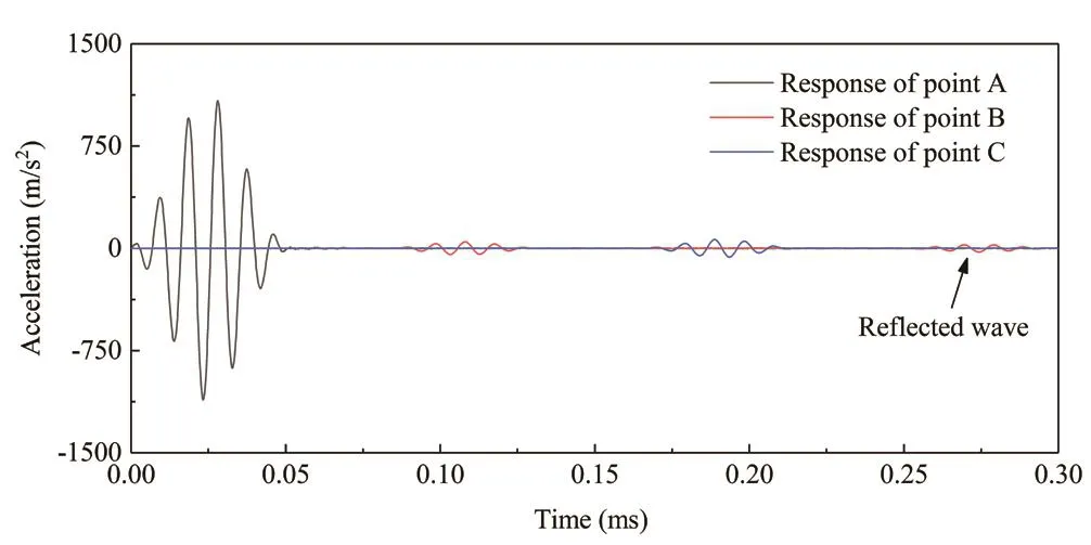
Fig.19 Response history of different points of the plate

Based on the derived quadrature scheme, several 1-D and 2-D structural elements are designed to solve problems concerning eigenvalue or transient analysis in structural dynamics.For natural vibration problems,in most cases the lumped-mass CSEM can behave as well as traditional consistent-mass CSEM.In addition,it exhibits much faster convergence than does classical FEM.For the simulation of elastic wave propagation in rod, beam and plate structures, the proposed method achieves satisfactory performance.Considering its high efficiency in conjunction with explicit time-marching schemes, the lumped-mass CSEM is thus more favorable than traditional consistent-mass CSEM for conducting large-scale dynamic analysis.

Acknowledgement

This work was supported in part by the Joint Research Fund for Earthquake Science launched by the National Natural Science Foundation of China and the China Earthquake Administration (Grant No.U2039208).The authors would like to thank research fellows Shaolin Chen in the College of Civil Aviation, Nanjing University of Aeronautics and Astronautics, and Zhenghua Zhou of the College of Transportation Engineering, Nanjing Tech University, for a fruitful discussion about the numerical technique of wave motion.