An optimized run-length based algorithm for sparse remote sensing image labeling

Shen-shen Luan, Bo-wen Cheng, Shuai Jiang, Yu-hang Wu, Zong-ling Li, Ji-yang Yu

Institute of Spacecraft System Engineering, Youyi Road, Haidian District, Beijing, China

Keywords:Connected-component labeling Label equivalence resolving Hardware implementation Equivalence matrix On-board processing

ABSTRACT Labeling of the connected components is the key operation of the target recognition and segmentation in remote sensing images. The conventional connected-component labeling (CCL) algorithms for ordinary optical images are considered time-consuming in processing the remote sensing images because of the larger size. A dynamic run-length based CCL algorithm (DyRLC) is proposed in this paper for the large size, big granularity sparse remote sensing image, such as space debris images and ship images. In addition, the equivalence matrix method is proposed to help design the pre-processing method to accelerate the equivalence labels resolving. The result shows our algorithm outperforms 22.86% on execution time than the other algorithms in space debris image dataset.The proposed algorithm also can be implemented on the field programming logical array(FPGA)to enable the realization of the real-time processing on-board.

1. Introduction

Labeling connected components is the fundamental operation method of the digital image processing[1],especially in the pattern and target recognition in remote sensing (RS). Many applications based on image analysis need connected-component labeling(CCL)algorithm as a pre-processing method, such as fingerprint identification, automated inspection, medical image analysis and target recognition. Now with the increase of the remote sensing image size and real-time processing application,faster CCL algorithms are always demanded to speed up the realization.

Many researches have been studied in decades for addressing the critical issue [1]. The CCL algorithms can be divided into five classes according to the computer architecture or data structure[1].The algorithms for ordinary computer architectures and twodimensional images are the most interested because they are the base of other algorithms, and can be divided into two types: algorithms based on label-propagation,and algorithms based on labelequivalence resolving [1]. F.Chang et al. proposed the contour tracing labeling (CTL) algorithm in 2004 to search the unlabeled border pixel firstly and then assign a new label to the component.Herrero[2]proposed the hybrid object labeling(HOL)algorithm by combining recursion with iterative scanning. The two algorithms above belong to the label-propagation. An optimized connectedcomponent labeling (OCL) algorithm is proposed by Wu et al., in 2009[3],which contains two optimization strategies to reduce the number of neighboring pixels accessed and track equivalence labels. He et al. [4] proposed an improved run-based CCL algorithm(IRCL) in 2010 to reduce the labeling time down to one and a half.And the IRCL algorithm can obtain contours of connected components efficiently. Decision trees are applied to optimize the blockbased CCL algorithm (BCL) by Grana in 2010 [5]. The BCL algorithm defined a new paradigm for eight-connection labeling by using OR-decision tables and a new scanning technique that covered a 2 × 2 pixel mask was used to scan the image. And Zhao et al. [6] proposed an improved configuration-transition-base algorithm (ICTCL), which scanned the image every three lines and processed pixels three by three. The four later algorithms are the label-equivalence resolving ones.

Recently the CCL algorithms have several new progresses in both the approach and implementation. Ravankar et al. [7] proposed a CCL algorithm for the sparse lidar data segmentation and used it to map the buildings from the lidar data in 2015. Schwenk et al. [8] proposed an implementation method of the two pass based CCL algorithm in 2015 for the very complex and high resolution images, which only need low memory consumption compared with the others. Yonehara et al. [9] presented a new parallel algorithm based on Union-find technique with GPU and the experiments on CUDA showed a 1.6x speedup than before in 2015.Laurent Cabaret et al.in Ref.[10,11]presented a parallel version of the Light Speed Labeling(LSL)algorithm and a SIMD RLE algorithm is proposed by Florian Lemaitre in 2020 in Ref.[12].For GPU based algorithm, Lacassagne L proposed a direct connected component labeling algorithm in Ref. [13] and block-based algorithm is optimized by Allegretti S et al.On GPU in Ref.[14].Cabaret proposed an efficient CCL algorithm for GPUs called Distanceless Label Propagation(DLP)in 2017[15].The LSL algorithm performed on a 4 x 15 core machine had a better performance and can achieve 42.4 gigapixel labels per second. Stamatovic [16] presented a labeling algorithm for 26-connected components in 3D binary lattices based on cellular automata algorithm.In Ref.[17],a labeling algorithm based on forest of decision trees is given to improve the neighborhood exploration in two-scan labeling. Compared with the method in Ref. [5], the mask proposed in the paper is smaller and makes the equivalent results. Federico Bolelli et al. [18] proposed a blockbased CCL algorithm using the model of Directed Rooted Acyclic Graph,which was called Spaghetti Labeling. In Ref. [18] the blockbased mask with state prediction and code compression was combined to improve the CCL algorithm performance and produced an extremely fast solution.

There are also some researches on the FPGA implementation of the algorithm. Crookes et al. [19] implemented the multi-pass connected component labeling algorithm on an FPGA using offchip RAM in 1999, but this implementation suffered from the problem with base algorithm and was time-consuming [20].Benkrid et al.[21]using Xilinx Virtex-E FPGA to implement the CCL algorithm to process 1024 x 1024 size of images and got the 68 pass/s performance. Jablonski et al. [22] implemented a CCL algorithm on the Xilinx FPGA with three steps: the segmentation and labeling,the label reordering and the label translation in 2004.The implementation is designed for 25fps with 512 x 512 images. For run-length based CCL algorithm, Kofi Appiah et al. [20] realize the FPGA implementation on Block RAM by parallel in 2008 and labeled a 720 x 576 size image in 0.017 s.Klaiber M J et al.realized a singlecycle parallel multi-slice CCL architecture in 2016 [23]. Bailey [24]proposed a Zig-Zag Based Single-Pass analyzing method. An embedded architecture was proposed by M. Tekleyohannes for industry application in 2017 [25].

The algorithms above are mostly proposed for the ordinary images, whose size is not too large and pixel density is homogeneous.Contrasted with the ordinary images,sparse remote sensing images have the features of large size, big granularity and low density, such as space debris images, ship images, island images and fractus images. For the RS image processing, there are two problems to be solved. Firstly, RS images are usually with a large size, while the on-board processing has a critically real-time requirement. The ordinary algorithms are considered timeconsuming when experimented on the large size images. Secondly, the algorithms for on-board processing should be suitable for the hardware implementation. The label propagation CCL algorithms mentioned above[2]access an image in an irregular way,which are not suitable for this requirement [1]. The algorithm for the RS images’ connected-components labeling should be specifically designed.

Based on the run-length algorithm [23], we proposed an improved CCL algorithm by pre-processing to resolve the label equivalences dynamically. Inspired with the sparse matrix, we turned the label equivalences into the equivalence matrix,which is proposed in this paper to help understand the process of the improved algorithm. The definition of the equivalence matrix is given in the Appendix A. When the label equivalence represented by the sparse matrix,we can find that the non-zero values(like 1s in Fig. 5(b)) of the equivalence matrix are distributed along the diagonal. Inspired by this feature, a pre-processing method before label equivalences resolving is proposed to decrease the search regions of the depth first searching(DFS)algorithm dynamically.So the looping number of DFS algorithm can be reduced efficiently.The pre-processing method can be realized by a serial operation of adding and subtracting simply, which is suitable for the hardware implementation. Our algorithm is proved to be faster than the conventional algorithm in labeling sparse remote sensing images as shown in section 5.

There are mainly two contributions in this paper. One is the equivalence matrix method,which help design the pre-processing method and analyze the other algorithms.The other one is the preprocessing method proposed for the large size, big granularity sparse remote sensing image labeling, which outperforms 22.86%on execution time than the other algorithms in the space debris image dataset.

In this paper, the first section introduces the conventional algorithms, the new requirements for CCL algorithm in remote sensing image processing, and the proposed algorithm’s feature.Section II demonstrates the conventional processing of run-length based CCL algorithm and its weakness in processing remote sensing images. The improved algorithm is proposed in section III by the equivalence matrix and pseudo-codes are listed to give a better understanding. And a mathematical model is established in section IV to analyze the proposed method theoretically. Experimental results are listed in the section V with comparison with other algorithms, and section VI gives the discussion about the efficiency of the proposed.Finally,the conclusion is given in the last section VII.

2. Previous work

In this section, the concept of connected component labeling will be introduced firstly to state the problem more clearly.Due to the requirement of the hardware implementation, the candidate algorithms are limited within the label equivalences resolving algorithms, which process the images in raster scan order and suitable for the streamed image data. For generating the label equivalences, there are two types of methods: the pixel-based[19,21,22,26,27] and the run-based [20, 28]. The proposed algorithm is based on the later, so here we then introduce the basic operation of the run-length based CCL algorithm.

2.1. Problem statement

For target segmentation and recognition of image analysis,connected component labeling is one of the most important basic operations. The labeling is operated on the binary image, so the gray/RGB images need to be transformed to binary images firstly.For the N x M binary image(N and M are the size of the image),the background pixels’ value are marked as 0, while the foreground pixels,which represent the object,are marked as 1.The connected component is the pixels which are neighbored with two categories:four-connected components and eight-connected components,shown as Fig. 1 (a) and (b). One connected component can be treated as one target and labeling, and all the connected components represents the different targets in one image.In Fig.1(c),the airport picture is taken as an example. There are 8 targets labeled from 1 to 8 which are distinguished by different colors.

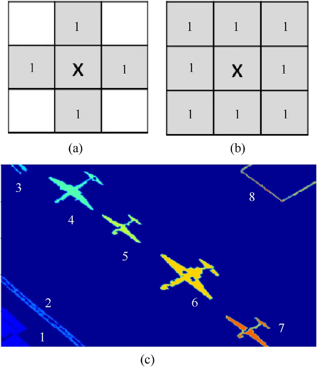
Fig. 1. Different connected components type. (a) Four-connected components; (b)Eight-connected components; (c) an example of labeled image. There are 8 labeled objects with different colors, four of them are airplanes.

As mentioned in section I,labeling the connected component is widely focused by many researchers and a lot of algorithms have been proposed in various applications to improve the efficiency.Different with the ordinary images, remote sensing images are usually with larger size and need to be processed on-board in realtime, which put up with a critical requirement on algorithm efficiency.So improvement or new CCL algorithms for remote sensing images must be studied to accelerate the processing.

2.2. Run-length based algorithm

There are three steps in the run-length based algorithm. The first step is to scan the image pixel by pixel to encode the runs and get the provisional labels.The second step is to scan the runs to get the label equivalences. And the last step is resolving the label equivalences by depth first search method to get the final label of the connected components. The three steps will be introduced in detail in the next three chapters.

2.2.1. Step 1: encoding runs and provisional labels

The scan is operated row by row,and a run is defined as a block of contiguous foreground pixels in a row, shown as Fig. 2. When scanning the image in the first time,the number of run,is recorded as the provisional label into run(i). The start pixel number of the run(i)is recorded into strun(i),and so as the end pixel number into enrun(i),the row number into rowrun(i).In conclusion,the row of run i is rowrun(i) and it’s spatial region in the image is [strun(i),enrun(i)], as shown in Fig. 2.

2.2.2. Step 2: Creating the label equivalence

After getting the provisional label, the second scan is used to create the label equivalences.The second scan starts from the runs in the second row and is operated between the adjacent rows.Here we discuss the eight-connected components’ processing. For run i and run j in the adjacent rows shown in Fig. 3(a), if enrun(i)＞=strun(j)-1 and strun(i)＜=enrun(j)+1,the run i is connected with run j by the eight-connected way. Without loss of generality, we can extend the judgment as (1), in which the offset is 1 for the eight-connection judging and 0 for the four-connection judging.

After the judgment of connection, the label of new connected component with two provisional labels should be updated with a new one.In other words,the label of run i and run j should be the same if the run i and run j is connected. Here the label of the new connected component is assigned with the smaller provisional label.If there are more than two runs connected,shown as Fig.3(b),the other runs’label are recorded with the smallest label as a pair,which is so called label equivalence. The label equivalences represent the connection relationship between runs after the second scan.

2.2.3. Step 3: Resolving the label equivalences

The label equivalences record the relationship of connected runs.For example,label equivalences such as(1,2)(2,4)(7,2)(1,5)(6,3)(8,3)means that run 1,2,4,5,7 are connected and run 3,6,8 are connected.Connected components should be assigned with the same label. So the final step of this algorithm is to resolve these label equivalences to get the united representative label.

Fig. 2. Encoding runs and assigning the provisional labels. The pixels with 1 mark are object pixels, and the blank pixels represent the background pixels. Run i is encoded with run(i), strun(i), enrun(i), rowrun(i). The provisional label is assigned into run(i). For example, the run in the second row (run j) is encoded with [run(j) = 4, strun(j) = 6,enrun(j) = 16, rowrun(j) = 2], and the provisional label is 4.

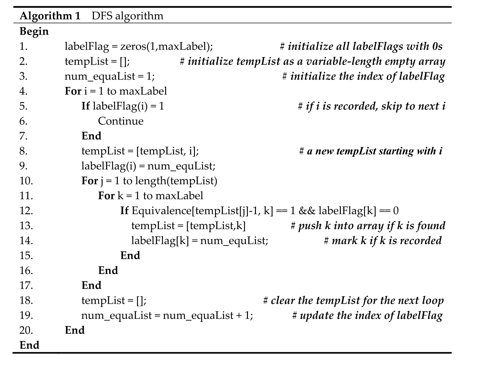
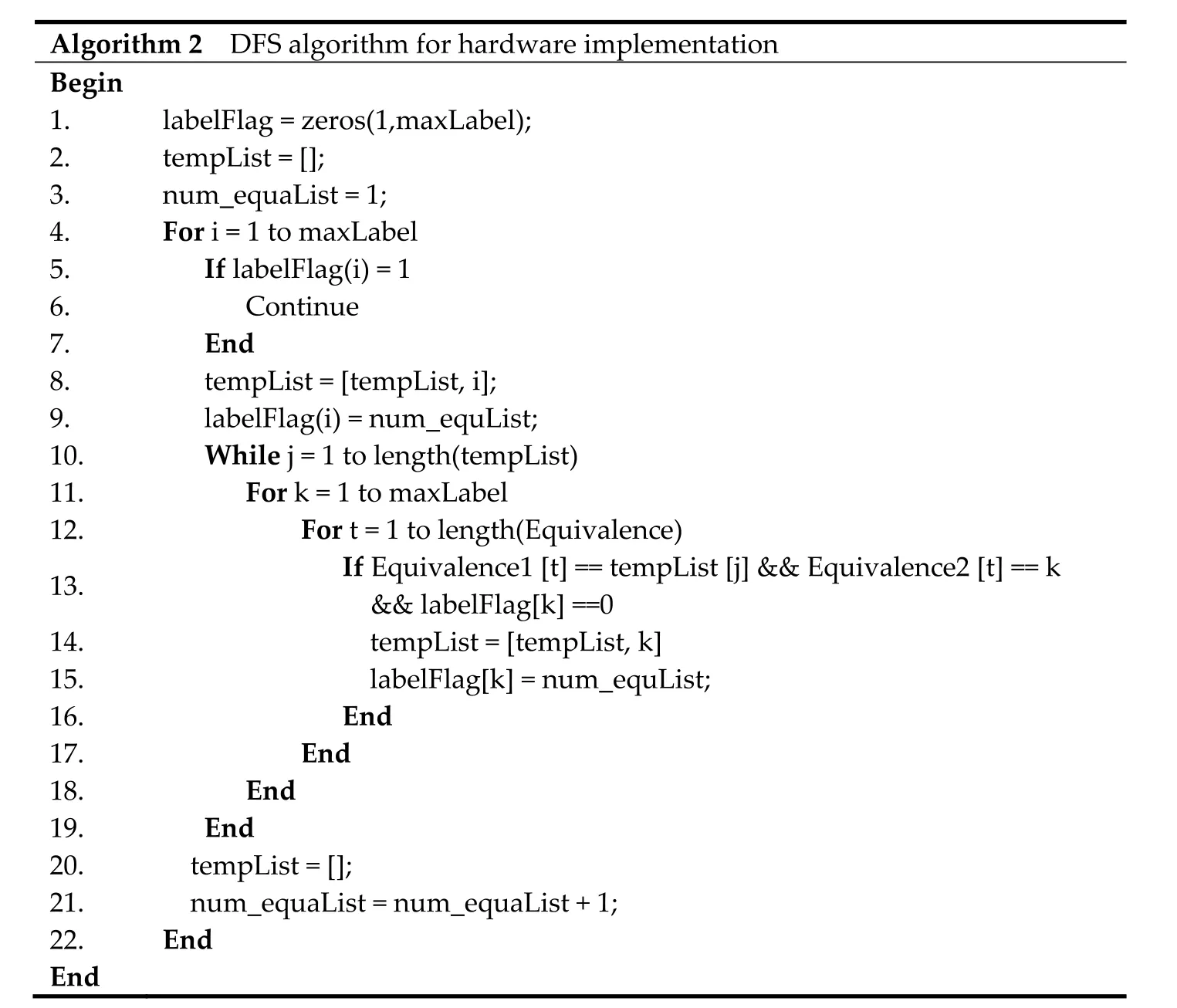
According to Ref. [29], the label equivalences resolving can be viewed as the undirected graph connecting according to the graph theory. Here the depth first search (DFS) method is used to solve this problem [30]. For the DFS method is a common algorithm in graph theory,we only give the pseudo-code written with MatLab as follows.into two arrays in Algorithm 2.tempList and labelFlag is the output of the DFS algorithm.

Generally speaking,there should be only three loops in the DFS’s pseudo-code, as shown in Algorithm 1. The algorithm enumerates all the label equivalences by looping i and k in the label equivalence(i, k) from 0 to maxLabel to match the real label equivalences. This

images/BZ_133_1254_1593_1271_1609.png

In Algorithm1, labelFlag records the state of whether the label has been recorded by tempList. Num_equiList records the index of the labelFlag, which is assigned to labelFlag to generate the final label. Equivalence represents the label equivalences by matrix,which is not suitable for hardware implementation and is changed step is realized by two loops in the first and eighth row in Algorithm 1. If there is a label equivalence matches, for example when i=1,k=3 and label equivalence(1,3)existing,it will be recorded into the array tempList(the 13th row in Algorithm 1).Once the label is recorded,it will not be checked again by setting its labelFlag(the 14th row and 5-7th row in Algorithm 1)to reduce the looping time.After this step, all the connected runs will be recorded by the tempList rather than label equivalence to make the real connected component. And all the labels in the same tempList have the same labelFlag (the 14th row in Algorithm 1). When the tempList for a certain i is completed,the tempList will be cleared(the 18th row in Algorithm 1) for the next loop(the 4th row in Algorithm 1). Fig. 4 shows an example of the processing of DFS method. There are two tempList [1,3,4,6], and [2,5,7], in which the labels are listed as the order of searching and popping down.row in Algorithm 2. Equivalence1 contains all the i in (i, k), and Equivalence2 contains all the k. The added loop (12th row of the Algorithm 2) enumerates the index in the two arrays to complete the search processing.It can be seen that the added loop will cause the increase of the time consuming,which is also discussed in the section VI.

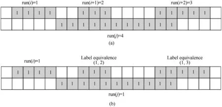
Fig. 3. The creating of the label equivalence: (a) The original provisional label of runs; (b) The run(j) has been assigned with run(i) when judging connection with run(i). And the other connected runs, like run(i+1)and run(i+2), have been recorded with the run(j) as the label equivalence (1,2) and (1,3).

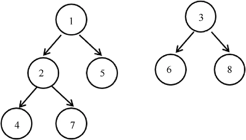
Fig.4. Two tempLists of DFS algorithm generated from(1,2)(2,4)(7,2)(1,5)(6,3)(8,3).According to the DFS algorithm,the searching order of the left templist is 1-2-4-7-5,and the right is 3-6-8.The labelFlag of label 1,2,5,4,7 is 1,and the labelFlag of label 3,6, 8 is 2.

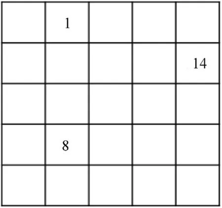
Fig. 5. The example of sparse matrix.

images/BZ_134_1236_2655_1253_2671.png

The 9th row of Algorithm 1 indicates that the judgment is operated on a matrix Equivalence, which is not suitable for the hardware implementation for large memory cost. So the matrix is rewritten as two arrays,Equivalence1 and Equivalence2,in the 13th

After the DFS algorithm, the label equivalences have been resolved into several tempLists. The label in the same tempList is connected and should be assigned with the same label.So it can be realized easily by replacing the labels in the tempList in order.The connected components labeling of all the runs is realized completely.

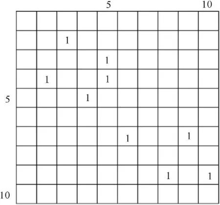
Fig. 6. The example of equivalence matrix. The label equivalences are(2, 3), (3, 5), (4,2), (4, 5), (5, 4), (7, 6), (7, 9), (9, 8), (9,10).

3. The equivalence matrix method

3.1. Definition and analysis

In mathematics,the sparse matrix is recorded by the array(row,column,value)other than the matrix to save the storage space.For example,the sparse matrix shown by Fig.5 is recorded by(1,2,1),(2, 5,14), (4, 2, 8).

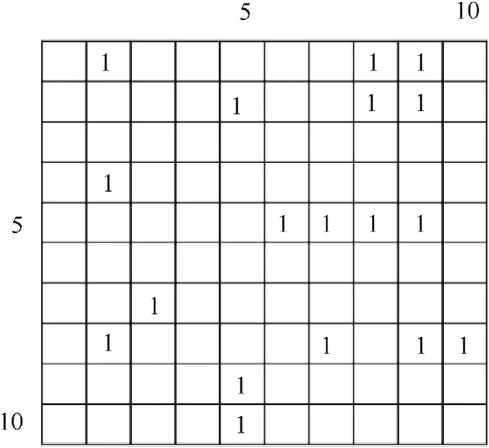
Fig. 7. Example for equivalence matrix with maxLabel = 10 and label equivalences of(1,2), (1,8), (1,9), (2,5), (2,8), (2,9), (4,2), (5,6), (5,7), (5,8), (5,9), (7,3), (8,2), (8,7), (8,9),(8,10), (9,5), (10,5).

For the label equivalences in this paper, it can be viewed that they are the recording of a sparse matrix with value of 1. So the matrix represented by the label equivalences is defined as the Equivalence Matrix. Here Fig. 6 shows an example of the representation of an equivalence matrix. The label equivalences are (2,3), (3, 5), (4, 2), (4, 5), (5, 4), (7, 6), (7, 9), (9, 8), (9,10).

So the algorithm above can be presented and analyzed by the equivalence matrix to give a better explanation of Step 3.

For a label equivalence(i,k),the maximum of i or k is maxLabel.So the size of equivalence matrix should be maxLabel * maxLabel.And all the elements of the equivalence matrix which match with the label equivalence (i, k) should be set as 1. Fig. 7 shows an example of equivalence matrix.

Taking Fig. 7 as an example, Algorithm 1 searches the equivalence matrix element one by one.The first loop(4th row)searches rows and the third loop (11th row) searches the column. The judgment operation (12-15th row) is repeated 100 times totally.Algorithm 2 searches the matrix by two arrays and the judgment operation(13-16th row)is also repeated 100 times totally.It can be seen that the operation time is proportional to maxlabel,which is the area of the equivalence matrix.

For remote sensing image,the bigger size of image may cause a bigger maxLabel. A bigger area of the equivalence matrix means more judgment to be operated and more time to cost.But if taking the equivalence matrix into a serious consideration,it can be found that there are a lot of zero elements in the matrix. Zero elements mean that there is no matching label equivalence and the judgment need not to be operated.So if we can reduce the searching area of the equivalence matrix instead of the whole area,the algorithm can save a lot of time.

By taking advantage of the big granularity feature of the sparse remote sensing images,we found a method to reduce the searching area of the equivalence matrix. And a pre-processing method inspired by equivalence matrix before the DFS was proposed,which will be demonstrated in IV.

3.2. Application on RS images

As mentioned above, the remote sensing binary images have two characteristics contrast with the ordinary optical binary images. Firstly, its size is larger, which means there are more provisional labels than ordinary images in probability. Secondly, the granularity of remote sensing binary images is usually bigger, in other words, the targets on remote sensing images are usually distributed locally and sparsely, such like space debris and ships.The localism and sparse characteristic determines that the two labels in one label equivalence is considered to have a smaller gap,such as(35,38)other than(35,68).Represented by the equivalence matrix, it can be seen that the 1 s in equivalence matrix is distributed along the diagonal, shown as Fig. 8(b). Here the equivalence matrixes of ordinary images and debris images are given in Fig. 8 to demonstrate the differences.

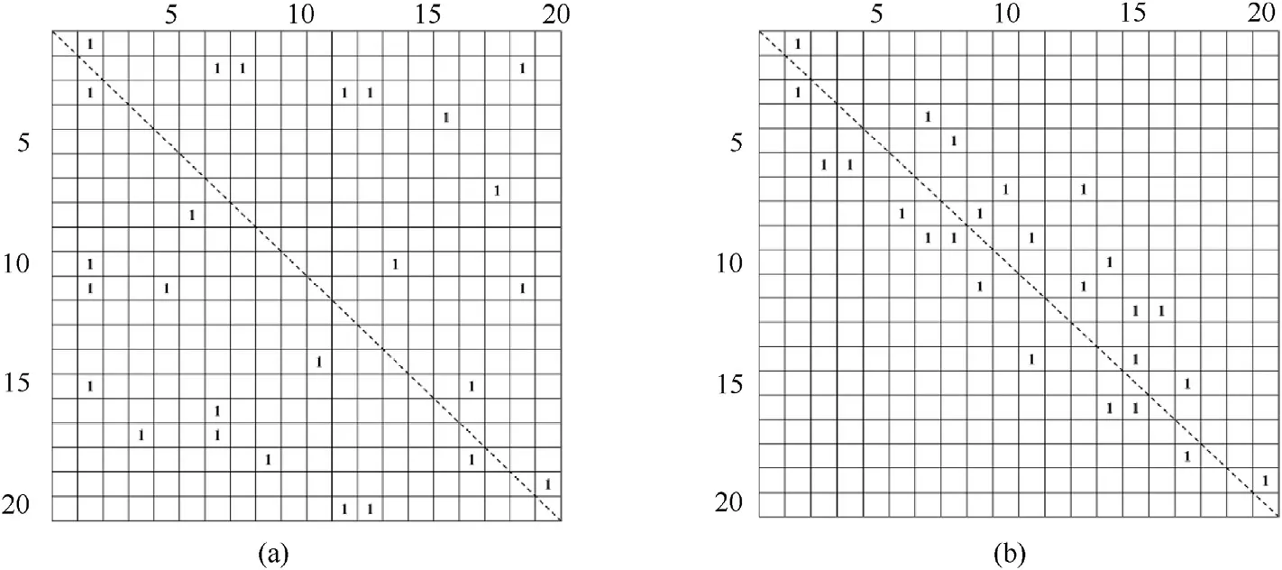
Fig. 8. The different distribution of 1s in equivalence matrix: (a) ordinary optical images; (b) remote sensing space debris images (images with big granularity).

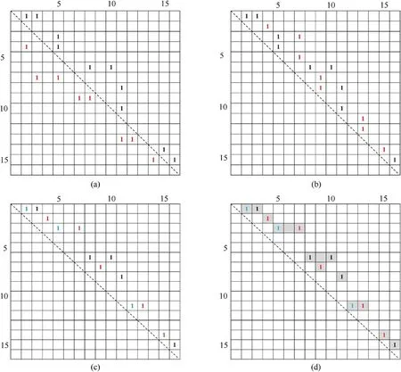
Fig. 9. The transformation of the equivalence matrix. (a) The original equivalence matrix in which the downer triangular elements are marked red; (b) The transformed upper triangular equivalence matrix in which red elements represent the transformation; (c) The transformed equivalence matrix by column 1s to row 1s in which the blue marked 1s represent the transformation; (d) The area with gray background is the search area for DFS algorithm after pre-processing method, contrast with the whole matrix area in (a) for original DFS algorithm.

As analyzed in chapter 2.3, to make sure matching all the label equivalence, the search area of DFS algorithm must cover all the matrix elements in Fig.8(a)to find all the 1s.This will be very time consuming when the matrix has a large size, such as remote sensing image.For the equivalence matrix shown as Fig.8(b),the 1s are distributed along the diagonal and there is no need to search all the matrix elements but only the limited area along the diagonal.This will abandon a lot of meaningless searches to save the time efficiently.In fact,the 1s area in Fig.8(b)can be reduced further by a pre-processing method and this will be introduced in the next section.

4. The proposed algorithm

4.1. Description

Fig.10. The processing of max_step and min_step. Equivalence_x and Equivalence_y reprensent the two elements of any label equivalence. Equivalence_y subtracted by Equivalence_x is the value of the step.For the same Equivalence_x,the max value of step is recorded as max_step and the minimum value is recorded as min_step.The gap is the length between the max_step and min_step.

The aim of the pre-processing method now is to limit the 1s searching area in equivalence matrix as much as possible.Inspired by the characteristic of label equivalence, there are three steps to realize the pre-processing method. Firstly, transform the matrix into the upper triangular matrix. Due to the label equivalence just represents the connection relationship between two runs,the label equivalence(x,y)equals to the label equivalence(y,x).So firstly we can change the x and y in label equivalence(x,y)to make sure x ＜y,which will change the equivalence matrix into the upper triangular matrix to reduce the search area,shown as Fig.9(a)and(b).In Fig.9(b),the 1s with red color is the symmetry result of that in Fig.9(a).It can be seen that the 1s area has been assembled further than before.

Secondly, transform ‘column 1s’ into ‘row 1s’ in the matrix. In the upper triangular matrix,there is condition that the 1s are listed in the same column,such as the 5th and 7th column,which is called‘column 1s’.The 1s listed in the same row is called‘row 1s’.Because the DFS method is operated with depth first, the middle 1s in the same column will be missed, which will result in the mistaken labeling.So the matrix must be transformed to change the column 1s to row 1s.

In the equivalence matrix,the 1s in the same column mean that the different runs represented by the different rows are connected by the same column. For example, in Fig. 9(b), there are 1s distributed in the 13th column, which is (11,13) and (12,13). For label equivalence, this means that run 11,12,13 are connected. So the label equivalences can be equally transformed into(11,12),(11,13), which does not change the connected relationship. The transformed 1s distribute in the same row shown in the 11th row in Fig. 9(c). After changing the column 1s into the row 1s, the DFS method is feasible again. The transformed result is shown in Fig. 9(c).

images/BZ_137_1099_2237_1116_2253.pngimages/BZ_137_1701_2237_1718_2253.pngimages/BZ_137_1236_2816_1253_2833.png

After the transformation of the equivalence matrix, the third step of the pre-processing method is to determine the range of search area.As shown in Fig.9(d),it is enough to set the search area within the elements with gray background to make sure completing searching all the connection relationship. Because the label equivalences are replaced by two arrays mentioned in chapter 2.2.3, here we give the discussion about how to realize the limitation of search area.

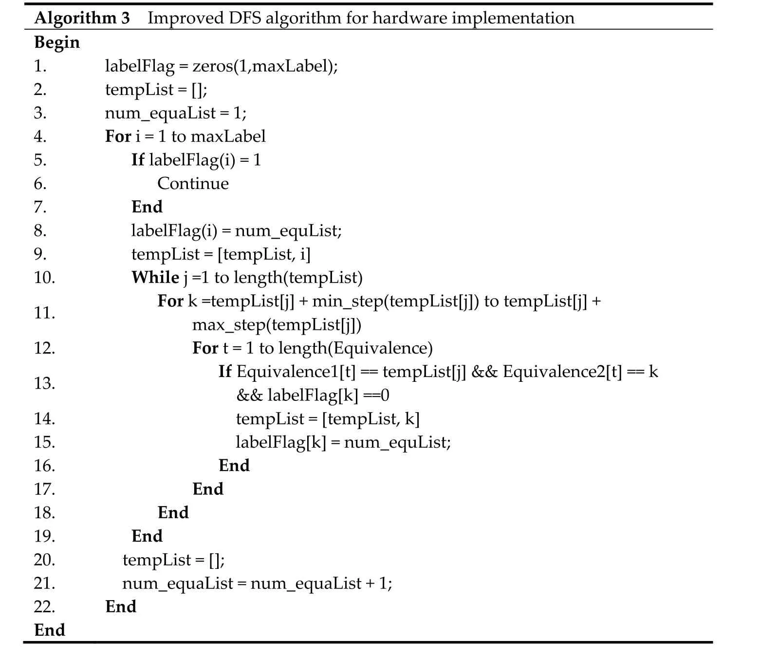
For a label equivalence (x, y), it has been recorded in array Equivalence_x and array Equivalence_y respectfully, shown in Fig.10. Taking x = 1 for an example, there are three label equivalences(1,2),(1,3)and(1,5).Undoubtedly,the searching row is the 1st row.The searching column here is from the 2nd column to the 5th column, which is not from 1st to maxLabel anymore. When it comes to algorithm realization, an array step is recorded with the distance between the x and y.max_step is the biggest value of the array step and the min_step is the smallest.The array max_step and min_step are used to control the search area in algorithm code.The array gap is used to measure the distance between the max_step and min_step, which will be used to calculate the efficiency in chapter 4.2.

After the three steps of pre-processing method (upper triangle transformation,column 1s to row 1s transformation and min-step/max-step recording), the DFS algorithm pseudo-code now can be modified as follows,in which the loop range has been changed from[0,run（i）] to [x + min-step, x + max-step] (the 8th row in the Algorithm 3). The search area of DFS algorithm has been reduced from the whole matrix into the smallest area, which is shown by the gray background in Fig. 9(d).

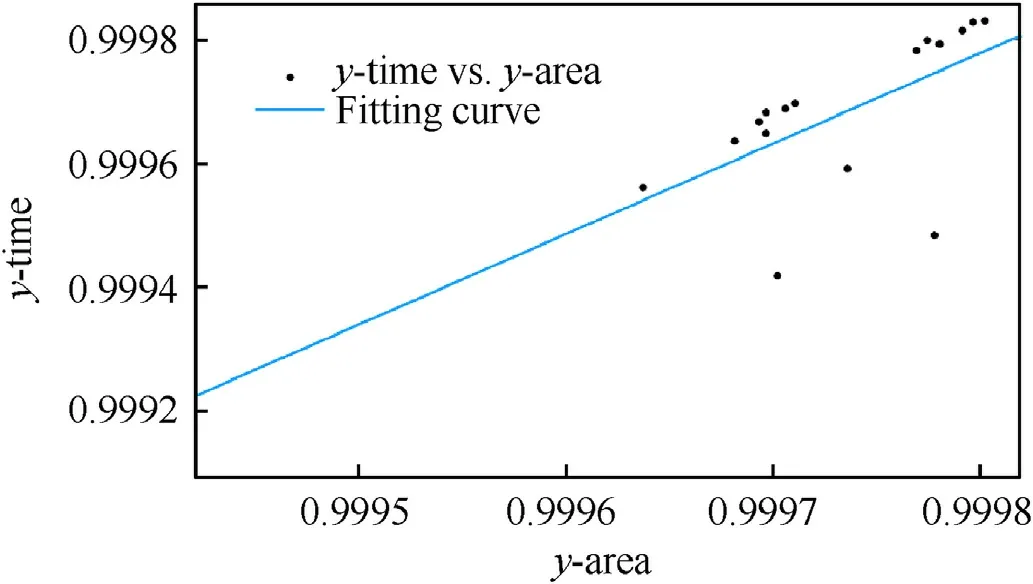
Fig. 11. The fitting results of the efficiency model. 16 experiments results have been fitted.The linear fitting model is y_time=1.462*y_area-0.4615,with RMSE 0.0001042 and R-square 0.3481.It can be seen that the time efficiency of the proposed algorithm can be calculated by the area of the equivalence matrix.

4.2. Theoretical analysis

4.2.1. The model of algorithm efficiency

In this section,a mathematical model will be given to verify the correctness of the proposed algorithm.According to section III,the loop times is proportional to the area of the equivalence matrix,so the efficiency model of the pre-processed DFS algorithm is established as follows.

In which γ is the efficiency of the model,N is the matrix size and Nrepresents the whole equivalence matrix area.gap is the search area of each provisional label and can be calculated by max_stepmin_step, as mentioned in chapter 4.1. ∑gap is the sum of all the gaps, which is equal to all the gray background searching area in equivalence matrix.In the original DFS algorithm,there is obviously∑gap =N.So the original DFS algorithm is set as the benchmark to calculate the efficiency here.

To verify this model, we compared the efficiency calculated by Eq.(2)and Eq.(3),which measures the efficiency directly from the operating time. tis the time of DFS algorithm with preprocessing method, and tmeans the original DFS algorithm without any pre-processing. Several experiments have been operated with MatLab and the results presents that the efficiency calculated by area and time are in good consistence and has a linear response, as shown in Fig.11. It also illustrates that the proposed equivalence matrix method is reasonable and feasible theoretically.

4.2.2. The complexity analysis

The time complexity of the proposed algorithm will be discussed in this section. There are mainly five operations in the proposed algorithm:

1.encoding the runs and assigning provisional label to the runs while scanning the image

2.creating equivalence labels while scanning the runs row by row

3.pre-processing the equivalence labels to record the search step

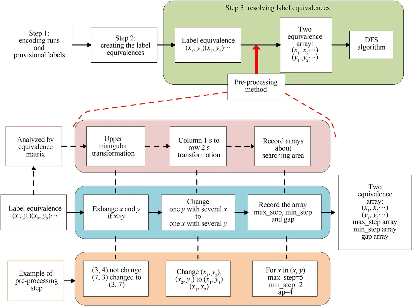
Fig.12. The flow chart of the proposed algorithms. on the top is the conventional algorithms proposed for ordinary optical images. The pre-processing method proposed in this paper is used in the step 3. The pre-processing method includes three steps, which are listed in the blue box. The proposed equivalence matrix is used to analyze the label equivalence and help design the pre-processing step by step,shown as the pink box.And the orange box shows an example of the pre-processing.The output of the preprocessing is five arrays.

4.resolving label equivalences by DFS to get the representative labels

5.replacing the provisional labels of runs with their representative labels

For an N×N pixel image,the maximum number of runs isN/4.So the maximum number of provisional labels or runs has an order ofO（N）.In our algorithm,it is obvious that procedure 1 and 5 have the order ofO（N）. In procedure 2, only constant operations are executed to creating equivalence label for each provisional label,so the order of procedure 2 should also be O（N） in the worst case.

The procedure 3 and 4 is used together for resolving the equivalence labels in the proposed algorithm. In the general DFS algorithm, there is only procedure 4 with no pre-processing method in procedure 3. To illustrate that the proposed procedure 3 can reduce the time complexity, we will calculate the order of only the procedure 4 existing firstly.

As mentioned above, to realize the hardware implementation,the loop of DFS algorithm has been extended from 3 to 4 times. It can be seen that the first two loop has an order of O（N）, and the third loop and fourth loop has an order of O（N）respectively.So the order when only the procedure 4 existing is O（N）.Accordingly,the order of the general DFS algorithm is O（N）.

Now the order of DFS algorithm with the pre-processing method will be calculated. The pre-processing method proposed in procedure 3 only contains constant operations such like subtracting or maximizing, so the order of procedure 3 can beO（N）in the worst case.But for procedure 4,due to the pre-processing of procedure 3,the third loop time is no more N,but a constant value far little than N. So the order of procedure 4 here is O（N）. Accordingly, the procedure 3 together with procedure 4 has an order of O（N）.

It can be found from the above discussion, our proposed algorithm has an order of O（N） contrast with the general DFS algorithm O（N）. The proposed algorithm has reduced the time complexity by the hardware implementation effectively.

5. Summary

In chapter 2.2, the run-length based algorithm is introduced with three steps and it is very time consuming when processing remote sensing images. To analyze the reason, we proposed the equivalence matrix method to analyze the run-length based algorithm in section 3.By this way,it is found that the looping times of the DFS algorithm are equal to the number of the equivalence matrix elements.The remote sensing images are usually with large size,which will result in a large number of looping times.This is the reason why it is extremely time consuming when processing the remote sensing images.

But in the same time, it is also found that the 1s in the equivalence matrix of the sparse remote sensing images are distributed along the diagonal in chapter 3.2, which is caused by the biggranularity of sparse remote sensing images. We can only search the 1s area of the equivalence matrix to reduce the looping times of algorithm.Inspired by this,a pre-processing method is proposed to limit the searching area within 1s area of the equivalence matrix,as shown in the top of Fig.12.

Table 1 The number of equivalences with image size 8192x8192.(X:granularity,Y:density,Content: the total number of 10 images).

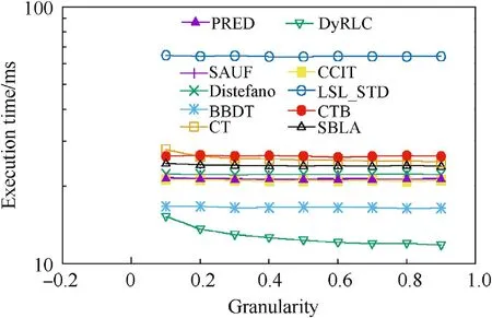
Fig.14. The average execution time of all the algorithms at different granularities with all sizes(density = 1%). Y-axis is set as log-style. The proposed DyRLC algorithm performs better than the others.

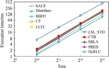
Fig. 15. The average execution time of all the algorithms at different sizes with all granularities(density = 1%). Y-axis is set log-style. The proposed DyRLC algorithm performs better than the other algorithms.

Fig.13. The samples of the 10 × 10, 20 × 20, 30 × 30 granularity images (from left to right) with size 1024 × 1024 and density 10%.

The pre-processing method includes three steps, which are all about the label equivalence operation, shown as the blue box in Fig. 12. The equivalence matrix here gives guidance and a better visualization of the three steps, shown as the pink box in Fig.12.The steps in blue box are equal to those in the pink box respectfully.And an example of the three steps is shown in the orange box in Fig.12. After the pre-processing method, the input data of DFS algorithm is augmented with three new arrays, max_step, min_step and gap. The three new arrays record the smallest areas of 1s in equivalence matrix. In other words, the three new arrays limit the looping times of DFS algorithm to the smallest.This pre-processing method also takes some time to be realized,but it is far fewer than the time wasted by the original algorithm.

In conclusion,the proposed equivalence matrix method acts the role of analysis and guidance of the proposed pre-processing method. It can also be used to analyze the other run-length based algorithms to improve their efficiency.

6. Experimental results

The dynamic run-length based algorithm is proposed specifically for the large size and big granularity sparse remote sensing binary images, so firstly the algorithm will be evaluated on the different size and different granularity image data. Then the real remote sensing image data set,with the targets of space debris and ship, will be used to evaluate the algorithm. The influence of the image density will also be experimented.

In order to propose a comparison with the state-of-the-art, we also performed several other algorithms on the dataset under the same situation. The algorithms we compared with are listed as follows,and the source code of all the algorithms was downloaded from the Github project YACCLAB-JRTIP[31-33],which is proposed by Federico Bolelli in Ref. [18].

• CT algorithm is the Contour Tracing approach by Fu Chang et al.,[2004]

• CCIT [34] is the algorithm by Wan-Yu Chang et al., [2015]

• DiStefano[35] is the algorithm by Di Stefano [1999]

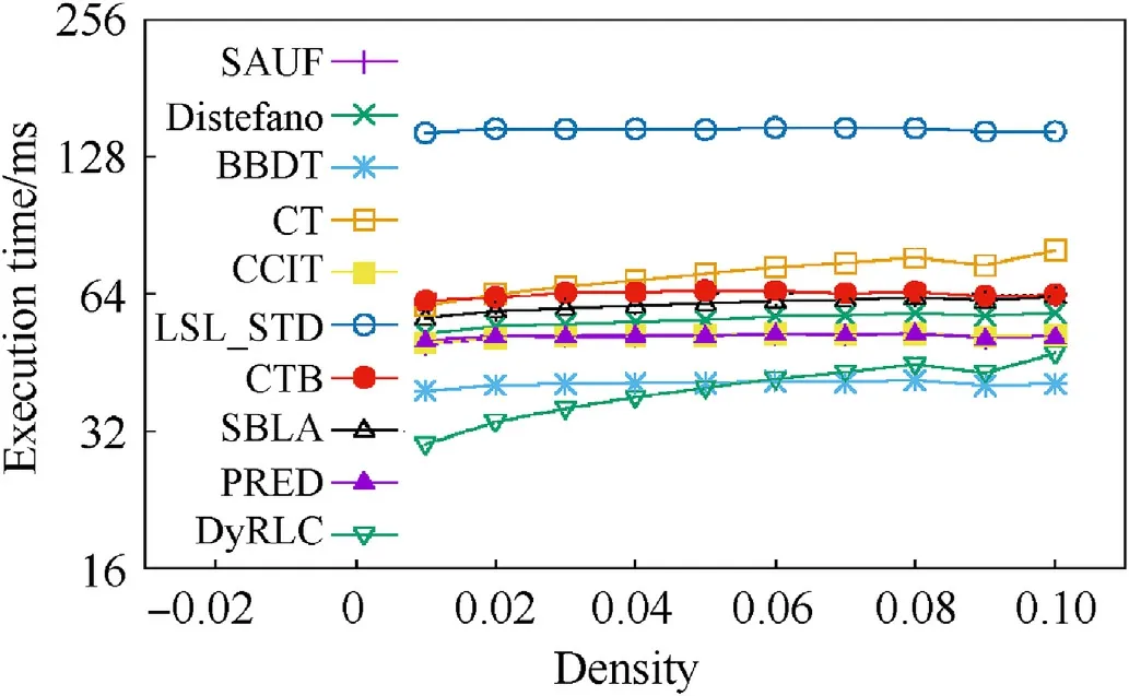
Fig.16. The average execution time of all the algorithms at different density with all granularities and sizes.Y-axis is set log-style.It can be seen that the propose algorithm performs best when the density is less than 6% and also better than all algorithms except for BBDT at all densities.

• BBDT [5] is the Block Based with Decision Trees algorithm by Grana et al., [2010]

• LSL STD[10]is the Light Speed Labeling algorithm by Lacassagne et al., [2016]

• SAUF [36] is the Scan Array Union Find algorithm by Wu et al.,[2009]

• CTB[37]is the Configuration-Transition-Based algorithm by He et al., [2014]

• SBLA [38] is the stripe-based algorithm by Zhao et al., [2010]

• PRED [39] is the Optimized Pixel Prediction by Grana et al.,[2016]

• DyRLC is the Dynamic Run-length Coding algorithm proposed in this paper

It is meaningless if there is any error labeling in the CCL algorithms. So there is no need to calculate the error rate of the algorithm. Any algorithm must label the connected components correctly.In our experiments,it is considered correct only when all the algorithms produce the same number of labels and the same labeling on the same images.All the experiments in this section are performed at least 10 times to average the execution time to remove possible outliers due to the other tasks performed by the operating system.The experiments were performed on the Lenovo ThinkCenter by using of an Intel(R) Core(TM) i7-6700 CPU @3.4 GHz processor and 16 GB RAM, and the operating system is Windows 10. The code is written in C++ and compiled on Windows using Visual Studio 2015.

6.1. Results on synthetic image dataset

As the other recent works, we produced a synthetic dataset of black and white random noise square images with nine different granularities,from a size of 1024×1024 pixels to a maximum size of 8192 × 8192 pixels. The granularities varied from 10 × 10 to 90 × 90 with a step of 10 pixels, shown in Fig.13. For every combination of size and granularity,10 images were produced for a total of 270 images. Besides, to illustrate the influence of the density of the images, we repeated producing the dataset 10 times with the density of its images varying from 1% to 10%. So finally there are 2700 images for this test.Table 1 shows the number of equivalences with image size 8192 × 8192.

Fig.14 shows how different algorithms behave with images with increasing granularity. The density of the images tested in this experiment is 1%. The reported value is the average time obtained considering all images with all granularities.It can be seen that our algorithm takes less time than the other algorithms at all the granularity. And the bigger the granularity is, the less time our proposed algorithm takes.

The second experiments proposed in Fig.15 shows the execution time of the algorithms with the different image sizes. The density of the images tested in this experiment is 1%.The reported value is the average time obtained considering all images with all sizes. A linear dependency of time on the size is shown for all algorithms and our algorithm performs well at each size.

Our approach proves to be scalable and performs well on different granularities.But for the CCL algorithm,the density of the images is another critical consideration.To illustrate the algorithms performance with different densities of the images, we tested all the algorithms on the image dataset with 1%-10% density respectfully. Fig. 16 shows the average execution time varying different densities. It can be seen that the proposed algorithm performs best than the other algorithms when the density is less than 6%,and also better than the algorithms at all densities except for BBDT. So the sparse feature plays an important role in the algorithm performance.The applications of our algorithm are mainly in the area of target detection on-board, and the images such as space debris,ships(on the sea),island,fractus,are all sparse remote sensing images.

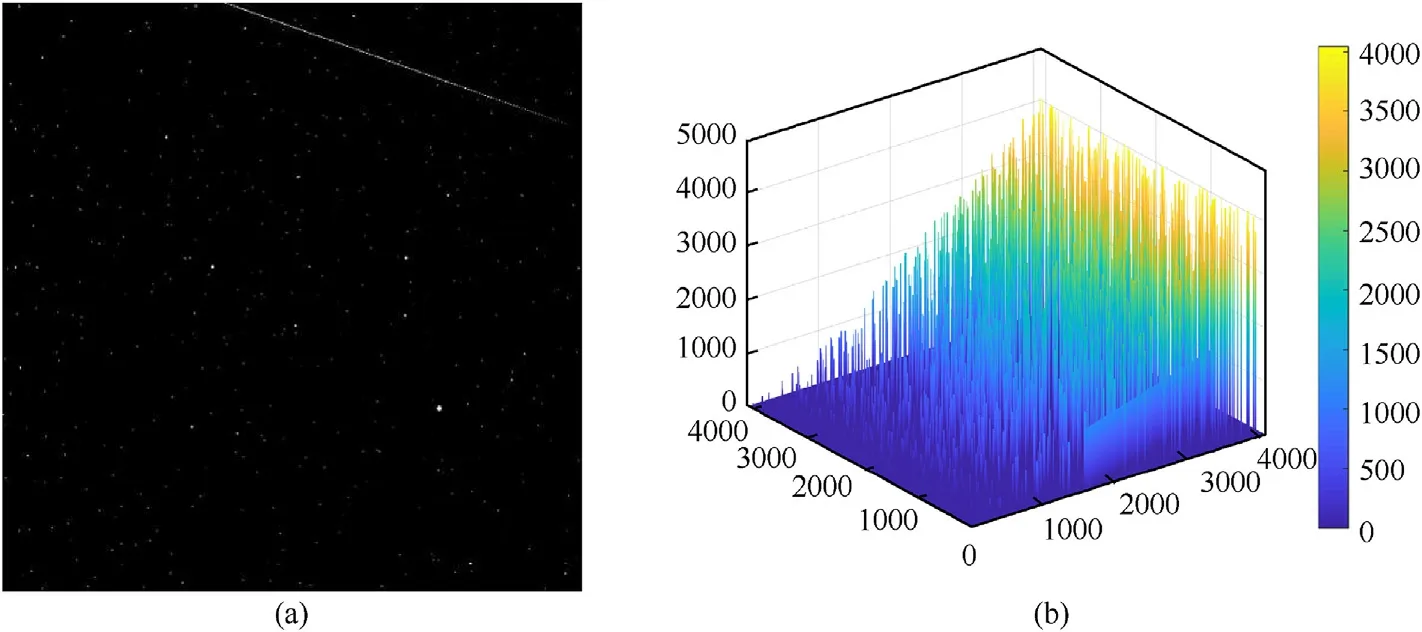
Fig.17. (a) The sample of the space debris image set. The white point can be the debris or the stars in the sky and the white line on the right-up area may be the noise of the telescope.(b)the result of labeling(a),the legend is the counting number of the connected components,which indicates that there are more than 4000 connected components in(a).

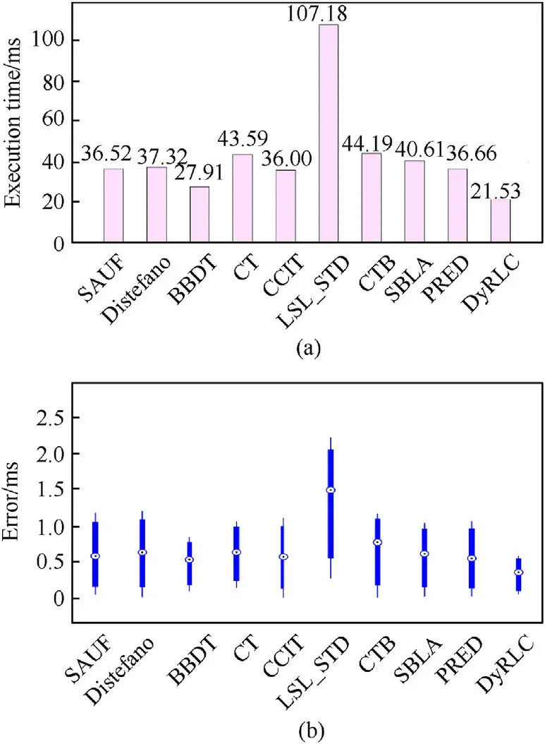
Fig.18. (a)The average execution time of all the algorithms on the space debris image set. The last one named DyRLC is our proposed algorithm; (b) The error of the algorithms, the black dot in the middle of the blue box is the root mean square error(RMSE), the upper edge and lower edge of the blue line represent the maximal error and minimum error respectively.

6.2. Results on sparse remote sensing image dataset

518 space debris images (4096 × 4096) as a dataset have been tested with repetition 10 times in this experiment. The debris image dataset is from National Astronomical Observatories of China and Fig. 17 (a) shows the sample of the dataset. The result oflabeling Fig. 17 (a) is shown in Fig. 17 (b). The average run-time performance of all the tested algorithms is shown in Fig. 18 (a).The error of the algorithms is shown in Fig. 18 (b), in which the black dot in the middle of the blue box is the root mean square error(RMSE) and the upper edge and lower edge of the blue line represent the max error and min error respectively. It can be seen that the proposed algorithm outperforms all other algorithms on the space debris dataset and has a 22.86% improvement on operating time.The proposed algorithm is in good stability as shown in Fig.18 (b).

Table 2The number of temporary labels, equivalences and final labels of the space debris images.

Table 2 shows the statistical data of the testing space debris images. It can be seen that although the space debris image is sparse, the number of the connected components is big enough because the large size of the remote sensing images.

For the optical remote sensing image, the special targets, such like clouds and ships,also have the feature of the large size and big granularity. So we also tested the algorithm on the ship image dataset from the GF2 remote sensing satellite, whose sample is shown in Fig.19.The dataset includes 90 images with size of 1024×1024. The result shown in Fig. 20 demonstrates that our proposed algorithm also performs well on ship recognition of large size RS images.

6.3. Results on hardware implementation

Monitoring the space debris and other time-vary targets onboard is a critical challenging mission for its real-time requirement. FPGA can be one of the best hardware solutions for satellite in this application due to its flexibility.Our proposed algorithm was also implemented in the FPGA to verify the feasibility and efficiency. The implementation is on Xilinx XC7V690T with four 8 Gb DDR3.

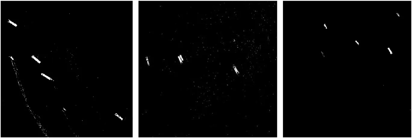
Fig.19. Three samples of the binary ship image set. The white areas represent the ships on the ocean.

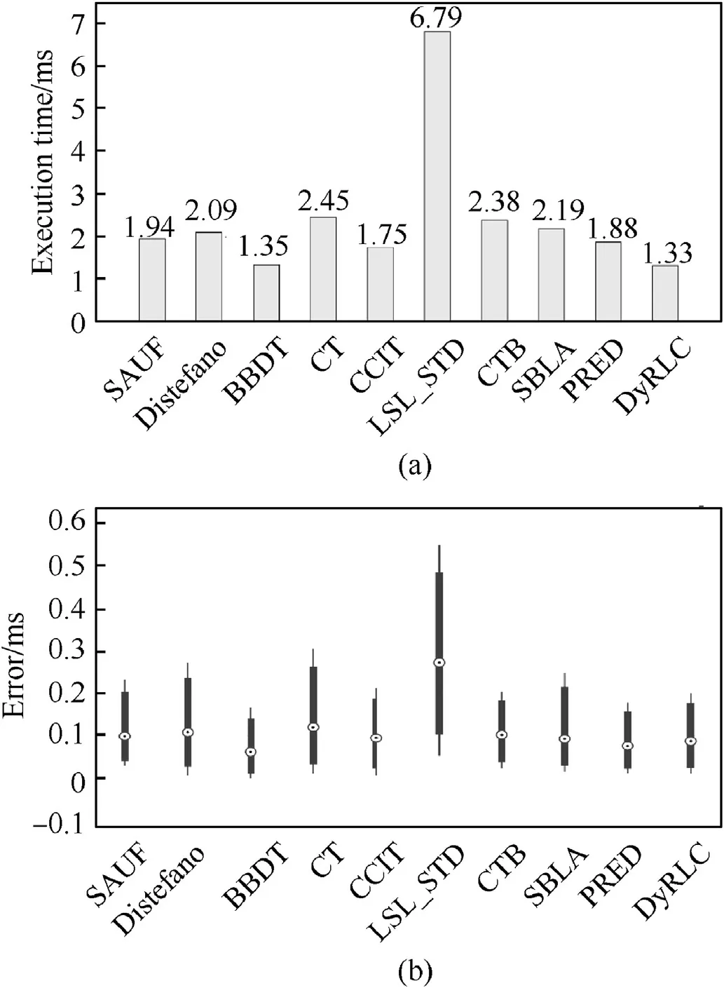
Fig.20. (a)The average execution time of all the algorithms on the ship image set.The last one named DyRLC is our proposed algorithm; (b) The error of the algorithms, the black dot in the middle of the blue box is the root mean square error(RMSE),the upper edge and lower edge of the blue line represent the maximal error and minimum error respectively.

As shown in Table 3,16 space debris images sampled from the above dataset had been tested with two algorithms, the CCL algorithm with original DFS method and our proposed algorithm with pre-processing DFS method, on the FPGA. It can be seen that the CCL algorithm with original DFS method takes about 10.715 s on average and is far from satisfying the real-time requirement. Our proposed algorithm only needs 0.122 s on average to label one space debris image,which improves the efficiency by 98.86%.Note that the image 15 and image 16 take a lot more time than the other 14 images,which causes the increase of the average time extremely.The reason is that the debris shape of image 15 and image 16 has a complex structure and causes a large number of label equivalences.In the real application,it cannot be avoided because of the different image qualities and the fixed binary processing method. But our proposed algorithm can deal with this problem very well for its processing time only increase 64.85% while the original DFS methods around 3600%.Besides,for the image 1-14,the proposed algorithm has a 95.50% improvement than the CCL algorithm with original DFS method on FPGA implementation. In addition, the implementation time of FPGA is more less than the non-FPGA platform shown in section 5.2, whose least time is 21.53 s while experimented on the same dataset.

Kofi Appiah et al. [20] realize the FPGA implementation on Xilinx Virtex-4 with 49.73 MHz and labeled a 720 x 576 size image in 0.017 s, which equals about 845410 clock cycles. In our implementation, a 4096 x 4096 space debris image is labeled in about 0.12184 s on Xlinx XC7V690T with 150 MHz, which equals about 18276000 clock cycles.It can be seen that our images size is 40.45 times larger than that of [20], the cycles of algorithm implementation of our algorithm is 21.62 times bigger than that of[20].

7. Conclusions

In this paper, we proposed a dynamic run-length based CCL algorithm for sparse remote sensing images, which outperforms than the conventional algorithms on the debris and ship dataset.With the increase of image size, especially for remote sensing images, the conventional algorithm is considered increasingly timeconsuming. Based on the run-length algorithm, we proposed a method of equivalence matrix to analyze the label equivalences and help optimize the algorithm. Taking advantage of the big granularity feature of sparse remote sensing images, the pre-processing method is designed before the DFS algorithm to resolve the equivalence labels more efficiently.

The pre-processing method mainly includes three steps,including exchanging labels, column 1s to row 1s transformation and recording searching area array. The output arrays help reduce the loop times of DFS algorithm and save a lot of time. The theoretical analysis of the proposed method is also performed by using the equivalence matrix. Experiments of synthetic image dataset and sparse remote sensing image dataset on both PC and FPGA arealso performed.The results show an obvious improvement than the other algorithms. It is proved that the proposed algorithm can be used on FPGA to realize the on-board processing.

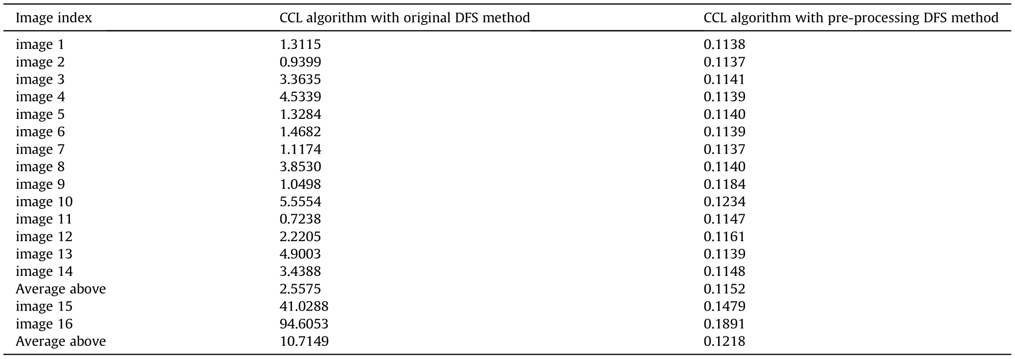
Table 3 The implementation time (unit:seconds) of the two algorithms on FPGA.

The authors declare no conflict of interest.