Deep learning for time series forecasting: The electric load case
2022-04-06AlbertoGasparinSlobodanLukovicCesareAlippi
Alberto Gasparin|Slobodan Lukovic|Cesare Alippi,2
1Faculty of Informatics, Università della Svizzera Italiana,Lugano, Switzerland
2Department of Electronics, Information, and Bioengineering,Politecnico di Milano,Milan, Italy
Abstract Management and efficient operations in critical infrastructures such as smart grids take huge advantage of accurate power load forecasting, which, due to its non-linear nature,remains a challenging task.Recently, deep learning has emerged in the machine learning field achieving impressive performance in a vast range of tasks,from image classification to machine translation.Applications of deep learning models to the electric load forecasting problem are gaining interest among researchers as well as the industry, but a comprehensive and sound comparison among different—also traditional—architectures is not yet available in the literature.This work aims at filling the gap by reviewing and experimentally evaluating four real world datasets on the most recent trends in electric load forecasting,by contrasting deep learning architectures on short-term forecast (oneday-ahead prediction).Specifically, the focus is on feedforward and recurrent neural networks, sequence-to-sequence models and temporal convolutional neural networks along with architectural variants, which are known in the signal processing community but are novel to the load forecasting one.
KEYWORDS deep learning, electric load forecasting, multi-step ahead forecasting, smart grid, time-series prediction
1|INTRODUCTION
Smart grids aim at creating automated and efficient energy delivery networks that improve power delivery reliability and quality, along with network security, energy efficiency, and demand-side management aspects [1].Modern power distribution systems are supported by advanced monitoring infrastructures that produce immense amount of data, thus enabling fine grained analytics and improved forecasting performance.In particular, electric load forecasting emerges as a critical task in the energy field,as it is of central relevance for a number of power distributions tasks at different levels of the grid.At the single-household level, accurate load forecasting can create savings opportunities while also help reduce the energy footprint.At a higher level in the grid (i.e., looking at the aggregated load from multiple households or buildings in general) electric load forecasting is a fundamental tool for power system operators as it provides support for different decision-making tasks such as the definition of better pricing strategies, the reduction of maintenance cost, improved demand-side management and efficient electrical energy storage management.Load forecasting is carried out at different time horizons, ranging from milliseconds to years, depending on the specific problem at hand.
Our main goal is to concisely review and assess the most appropriate deep learning models that could be utilised in the smart grid field specifically for load forecasting.In this work,we focus on the day-ahead prediction problem also referred to in the literature asshort-term load forecasting(STLF)[2].Since deregulation of electric energy distribution and wide adoption of renewables strongly affects daily market prices, STLF emerges to be of fundamental importance for efficient power supply [3].Furthermore, we differentiate forecasting on the granularity level at which it is applied.For instance, in an individual household scenario,load prediction is a rather difficult task as power consumption patterns are highly volatile.Thus,despite not being a very relevant task from the perspective of smart grids,we consider it for the sake of testing the proposedmodels with challenging and noisy dynamics.On the contrary,aggregated load consumption, that is, that associated with a neighbourhood, a region, or even an entire state, is normally easier to predict as the resulting signal exhibits slower dynamics.Still, the problem remains extremely relevant for the industry as even a small—statistically sound—increase in prediction accuracy can be translated into significant savings.
Historical power loads are time series affected by several external time variant factors,such as weather conditions,human activities, type of industrial processes, temporal and seasonal characteristics, which make their predictions a challenging problem.A large variety of prediction methods has been proposed for electric load forecasting over the years,and only the most relevant ones are reviewed in this survey.Autoregressive moving average models (ARMA) were among the first model families used in short-term load forecasting [4, 5].Soon they were replaced by autoregressive-integrated moving average(ARIMA) and seasonal ARIMA models [6] to cope with time variance often exhibited by load profiles.In order to include exogenous variables like temperature into the forecasting method, the autoregressive moving average model with eXogenous inputs(ARMAX)[7,8]and the autoregressive-integrated moving average model with eXogenous inputs (ARIMAX) [9]were introduced.The main shortcoming of these system identification families is the linearity assumption for the system being observed, a hypothesis that does not generally hold.In order to solve this limitation, non-linear models like feedforward neural networks were proposed and became attractive for those scenarios exhibiting significant non-linearity,as in load forecasting tasks[3,10-13].The intrinsic sequential nature of time series data was then exploited by considering sophisticated techniques ranging from advanced feed-forward architecture with residual connections [14] to convolutional approaches[15,16]and recurrent neural networks[17,18]along with their many variants such as the echo-state network[18-20],long short-term memory [18, 21-23] and gated recurrent unit[18, 24].Moreover, some hybrid architectures have also been proposed,aiming to capture the temporal dependencies in the data with recurrent networks while performing a more general feature extraction operation with convolutional layers[25,26].
Different surveys address the load forecasting topic by means of (not necessarily deep) neural networks.In [42], the authors focus on the use of some deep learning architectures for load forecasting.However, this review lacks a comprehensive comparative study of performance verified on common load forecasting benchmarks.The absence of valid costperformance metric does not allow the report to make conclusive statements.In [18], an exhaustive overview of recurrent neural networks for short-term load forecasting is presented.The very detailed work considers one-layer (not deep) recurrent networks only.A comprehensive summary of the most relevant research dealing with short-term load forecasting (STLF) employing recurrent neural networks, convolutional neural networks and seq2seq models is presented in Table 1.It emerges that most of the works have been performed on different datasets,making it rather difficult—if not impossible—to assess their absolute performance and,consequently,recommend the best state of the art solutions for load forecasting.
In this survey, we consider the most relevant—and recent—deep architectures and contrast them—also not on deep models—in terms of performance accuracy on opensource benchmarks.The considered architectures include linear models,shallow and deep feed-forward neural networks,recurrent neural networks, sequence-to-sequence models and temporal convolutional neural networks.The experimental comparison is performed on four different real world datasets that are representatives of two distinct scenarios.Three datasets consider power consumption at an individual household level with a signal characterised by high-frequency components while the last dataset takes into account aggregation of several consumers.
Our contributions consist in the following:
●A comprehensive review.The survey provides a comprehensive investigation of deep learning architectures known to the smart grid literature as well as novel recent ones suitable for electric load forecasting.
●A multi-step prediction strategy comparison for recurrent neural networks: we study and compare how different prediction strategies can be applied to recurrent neural networks.To the best of our knowledge,this work has not been done yet for deep recurrent neural networks.
●A relevant performance assessment.To the best of our knowledge, the present work provides the first systematic experimental comparison of the most relevant deep learning architectures for the electric load forecasting problems of individual and aggregated electric demand.It should be noted that the envisaged architectures are domain-independent and,as such,can be applied in different forecasting scenarios.In order to make the experiments reproducible—a very important aspect not rarely underestimated—all datasets used in this survey,as well as the source code,are publicly available.
The rest of this work is organised as follows:
In Section 2, we formalise the forecasting problem along with the notation that will be used in this work.In Section 3,we introduce feed-forward neural networks (FNNs) and the main concepts relevant to the learning task.We also provide a short review of the literature regarding the use of FNNs for the load forecasting problem.
In Section 4,we sketch recurrent neural networks(RNNs)and overview their most advanced architectures: long shortterm memory and gated recurrent unit networks.
In Section 5,sequence-to-sequence architectures(seq2seq)are discussed as a general improvement over recurrent neural networks.We present both, simple and advanced models built on the sequence-to-sequence paradigm.
In Section 6,convolutional neural networks are introduced,and one of their most recent variants, the temporal convolutional network (TCN), is presented as the state-of-the-art method for univariate time series prediction.

T A B L E 1 A summary of prior works that address the topic of electric load forecasting with deep learning models
In Section 7, the real world datasets used for the models'comparison are presented.For each dataset, we provide adescription of the preprocessing operations and the techniques that have been used to validate the models' performance.
Finally, In Section 8, we draw conclusions based on performance.
2|PROBLEM DESCRIPTION
In basic multi-step-ahead electric load forecasting,a univariate time series s=[s[0],s[1]…,s[T]] that spans through several years is given.Input data are presented to the different predictive families of models as a regressor vector composed of fixed time-lagged data associated with a window size of lengthnT, which slides over the time series.The size of the time window is a hyperparameter whose optimal value has to be identified on the data at hand.Given this fixed length view of past values,a predictorfaims at forecasting the nextnOvalues of the time series.In this work,the forecasting problem is cast into a supervised learning problem.As such, given the input vector at discrete timetxt=[s[t-nT+1],…,s[t]]∈IRnT,the forecasting problem requires to infer the nextnOmeasurements yt=[s[t+1],…,s[t+nO]]∈IRnOor a subset of it.To ease the notation, we express the input and output vectors in the reference system of the time window (relative time)instead of the time series one(absolute time).By following this approach, the input vector at discrete timetbecomes xt=[xt[0],…,xt[nT-1]]∈IRnT,xt[i]=s[i+1+t-nT] and the corresponding output vector is yt=[yt[nT-1],…,yt[nT+nO-2]]∈IRnO.ytcharacterises the real output values defined asyt[t]=xt[t+1],∀t∈T.Similarly, we denote asthe prediction vector provided by a predictive modelfwhose parameters vector Θ has been estimated by optimising a performance function.
Without loss of generality,in the remainder of the work,we drop the subscripttfrom the inner elements of xtand yt.The introduced notation, along with the sliding window approach,is depicted in Figure 1.
In certain applications, we will additionally be provided with extrad-1 exogenous variables (e.g., the temperatures),each of which represent a univariate time series aligned in time with the data of electricity demand.In this scenario,the components of the regressor vector become vectors,that is, xt=[x[0],…,x[nT-1]]∈IRnT×d.Indeed, each element of the input sequence is represented as x[t]=[x[t],z0[t],…,zd-2[t]]∈IRd, wherex[t]∈IR is the scalar load measurement at timet, whilezk[t]∈IR is the scalar value of thekthexogenous feature.
The nomenclature used in this work is given in Table 2.
3|FEED-FORWARD NEURAL NETWORKS
Feed-forward neural networks (FNNs) are parametric model families characterised by the universal function approximation property [43].The computational architectures are composed of a layered structure consisting of three main building blocks: the input layer, the hidden layer(s) and the output layer.The number of hidden layers (L>1), determines the depth of the network, while the size of each layer, that is, the numbernH,ℓof hidden units of theℓ-th layer defines its complexity in terms of neurons.FNNs provide only direct forward connections between two consecutive layers, each connection associated with a trainable parameter; note that given the feed foward nature of the computation, no recursive feedback is allowed (as it happens instead in recurrent networks).More in detail, given a vector x ∈IRnTfed at the network input, the FNN's computation can be expressed as

where h0=xt∈IRnTand ^yt=hL∈IRnO.
Each layerℓis characterised by its own parameters'matrix Wℓ∈IRnH,ℓ-1×nH,ℓand bias vector bℓ∈IRnH,ℓ.Hereafter, in order to ease the notation,we incorporate the bias term in the weight matrix, that is, Wℓ=[Wℓ;bℓ] and hℓ=[hℓ;1].Θ=[W1,…,WL] groups all the network's parameters.
Given a training set ofNinput-output vectors in the (xi,yi) form,i=1,…,N, the learning procedure aims at identifying a suitable configuration of parametersthat minimises a loss function L(Θ) evaluating the discrepancy between the estimated valuesf(xt;Θ) and the measurement yt:

The mean squared error,

is a very popular loss function for time series prediction; not rarely, a regularisation penalty term is introduced to guide the minimisation (learning) procedure towards solution incorporating some wished property, for example, predictor smoothness as well as mitigating occurrence of model overfitting.

The most used regularisation scheme controlling model complexity is the L2 regularisation Ω(Θ)=λ‖, beingλa suitable hyperparameter controlling the intensity of the regularisation.
As Equation (4) is not convex, the solution cannot be obtained in a closed form with linear equation solvers or convex optimisation techniques.Parameter estimation(learning procedure) operates iteratively for example, by leveraging on the gradient descent approach:
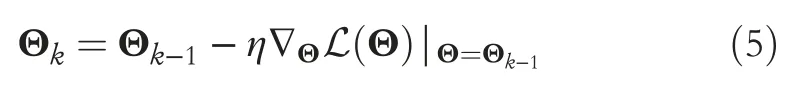
whereηis the learning rate and ∇ΘL(Θ) the loss function gradient with respect to Θ.Stochastic gradient descent,RMSProp [44], Adagrad [45], Adam [46] are popular learning procedures.The learning procedure yields estimate=Θkassociated with the predictive modelf(xt;).
Here, we consider deep FNNs to be the baseline architectures.
In multi-step-ahead prediction,the output layer dimension coincides with the forecasting horizonnO>1.The dimension of the input vector depends also on the presence of exogenous variables; this aspect is further discussed in Section 7.
3.1|FNNs' application for short-term load forecasting
The use of feed-forward neural networks in short-term load forecasting dates back to the 90s.Authors in [11] propose a shallow neural network with a single hidden layer to provide a 24-h forecast using both load and temperature information.In[10], one-day-ahead forecast is implemented using two different prediction strategies: one network provides all 24 forecast values in a single shot(MIMO strategy)while another single output network provides the day-ahead prediction by recursively feedbacking its last value estimate (recurrent strategy).The recurrent strategy proves to be more efficient in terms of both training time and forecasting accuracy.In [47],the authors present a feed-forward neural network to forecast electric loads on a weekly basis.The sparsely connected feedforward architecture receives the load time series, temperature readings,as well as the(coded)time and day of the week.It is shown that the extra information improves the forecast accuracy compared to an ARIMA model trained on the same task.[12]presents one of the first multi-layer FNNs to forecast the hourly load of a power system.
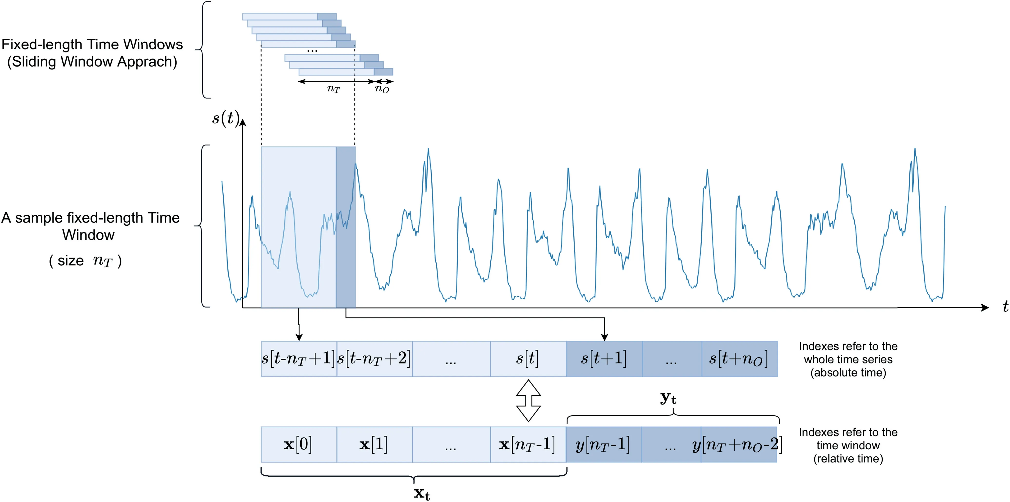
F I G U R E 1 A sliding windowed approach is used to frame the forecasting problem into a supervised machine learning problem.The target signal s is split in multiple input output pairs (xt,yt)∀t ∈{nT,nT+1,…,T-n0}
A detailed review concerning applications of artificial neural networks in short-term load forecasting can be found in[3].However, this survey dates back to the early 2000s and does not discuss deep models.More recently, architectural variants of feed-forward neural networks have been used; for example, in [14], a ResNet [48] inspired model is used to provide day-ahead forecast by leveraging on a very deep architecture.The article shows a significant improvement on aggregated load forecasting when compared to other (not neural) regression models on different datasets.
4|RECURRENT NEURAL NETWORKS
In this section, we overview recurrent neural networks and,in particular, the Elmann Net architecture [49], long short-term memory [50] and the gated recurrent Unit [51] networks.Afterwards, we introduce deep recurrent neural networks and discuss different strategies to perform multi-step-ahead forecasting.Finally, we present related work in short-term load forecasting that leverages on recurrent networks.
4.1|Elmann RNNs
Elmann recurrent neural networks (ERNN) were proposed in[49] to generalise feed-forward neural networks for better handling ordered data sequences like time series.
The reason behind the effectiveness of RNNs in dealing with sequences of data is their ability to learn a compact representation of the input sequence xtby means of a recurrent functionfthat implements mapping:

The architecture is depicted in Figure 2.
By expanding Equation (6) and given sequence xt=[x[0],…,x[nT-1]], x[t]∈IRdthe neural computation satisfies the following equation:

where W ∈IRnH×nH,U ∈IRd×nH,V ∈IRnH×nOare the weight matrices for hidden-hidden, input-hidden, and hidden-output connections, respectively,φ(·) is an activation function(generally the hyperbolic tangent one) andψ(·) is normally a linear function.The computation of a single module in an Elmann recurrent neural network is depicted in Figure 3.
It can be noted that an ERNN processes one element of the sequence at a time,preserving its inherent temporal order.After reading an element from the input sequence x[t]∈IRd,the network updates its internal state h[t]∈IRnHusing both(a transformation of) the latest state h[t-1] and (a transformation of) the current input (Equation 6).The described process can be better visualised as an acyclic graph obtained from the original cyclic graph (left side of Figure 2) via an operation known as time unfolding(right side of Figure 2).It is of fundamental importance to point out that all nodes in the unfolded network share the same parameters, as they are just replicas distributed over time.

T A B L E 2 The nomenclature used in this work
The parameters of the network Θ=[W,U,V] are usually learnt via backpropagation through time (BPTT) [52, 53], a generalised version of standard backpropagation.In order to apply gradient-based optimisation, the recurrent neural network has to be transformed through the unfolding procedure shown in Figure 2.In this way,the network is converted into a FNN having as many layers as time intervals in the input sequence,and each layer is constrained to have the same weight matrices.In practice, truncated backpropagation through time[54] (TBPTT) (τb,τf) is used.The method processes an input window of lengthnTone timestep at a time and runs BPTT forτbtimesteps everyτfsteps.Notice that havingτb<nTdoes not limit the memory capacity of the network as the hidden state incorporates information taken from the whole sequence.Despite that, settingτbto a very low number may result in poor performance.In the literature, BPTT is considered equivalent to TBPTT (τb=nT,τf=1).In this work, we used epoch-wise truncated BPTT that is, TBPTT(τb=nT,τf=nT) to indicate that the weights' update is performed once a whole sequence has been processed.

F I G U R E 2 (Left) A simple RNN with a single input.The black box represents the delay operator which leads to Equation (6).(Right) The network after unfolding.Note that the structure reminds that of a (deep)feedforward neural network but,here,each layer is constrained to share the same weights.hinit is the initial state of the network which is usually set to zero
Despite the model simplicity, Elmann RNNs are hard to train due to the ineffectiveness of gradient (back)propagation.In fact, it emerges that the propagation of the gradient is effective for short-term connections but is very likely to fail for long-term ones, when the gradient norm usually shrinks to zero or diverges.These two behaviours are known as the vanishing gradient and the exploding gradient problems[55, 56] and are extensively studied in the machine learning community.
4.2|Long short-term memory
Recurrent neural networks with long short-term memory(LSTM) were introduced to cope with the vanishing and exploding gradients'problems occurring in ERNNs and,more in general, in standard RNNs [50].LSTM networks maintain the same topological structure of ERNN but differ in the composition of the inner module—or cell.
Each LSTM cell has the same input and output as an ordinary ERNN cell but, internally, it implements a gated system that controls the neural information processing (see Figures 3 and 4).The key feature of gated networks is their ability to control the gradient flow by acting on the gate values; this allows the learning procedure to tackle the vanishing gradient problem, as LSTM can maintain its internal memory unaltered for long time intervals.Notice from the equations below that the inner state of the network results as a linear combination of the old state and the new state (Equation 14).Part of the old state is preserved and flows forward while in the ERNN, the state value is completely replaced at each timestep (Equation 8).In detail, the neural computation is

F I G U R E 3 A simple Elmann recurrent neural network block with one cell implementing Equation (7) and (8) once rewritten as matrix concatenation:a[t]=[W,U]T[h[t-1],x[t]],h[t]=φ(a[t]), with [W,U]∈IR(nH+d)×nH and [h[t-1],x[t]]∈IRnH+d, Usually φ(·) is the hyperbolic tangent


where Wf,Wi,Wo,Wc∈IRnH×nH, Uf,Ui,Uo,Uc∈IRnH×dare parameters to be learnt,⊙is the Hadamard product,ψ(·)is generally a sigmoid activation whileφ(·)can be any non-linear one (hyperbolic tangent in the original paper).The cell state c[t] encodes the—so far learnt—information from the input sequence.At timestept, the flow of information within the unit is controlled by three elements called gates:the forget gate f[t] controls the cell state's content and changes it when obsolete,the input gate i[t]controls which state value and how much will be updated,~c[t],finally the output gate o[t]produces a filtered version of the cell state and serves it as the network's output h[t] [57].
4.3|Gated recurrent units
First introduced in [51], gated recurrent units (GRUs) are a simplified variant of LSTM and, as such, belong to the family of gated RNNs.GRUs distinguish themselves from LSTMs for merging in one-gate functionalities controlled by the forget gate and the input gate.This kind of cell ends up having just two gates, which results in a more parsimonious architecture compared to LSTM that, instead, has three gates.
The basic components of a GRU cell are outlined in Figure 5, whereas the neural computation is controlled by:

F I G U R E 4 Long-Short Term Memory block with one cell
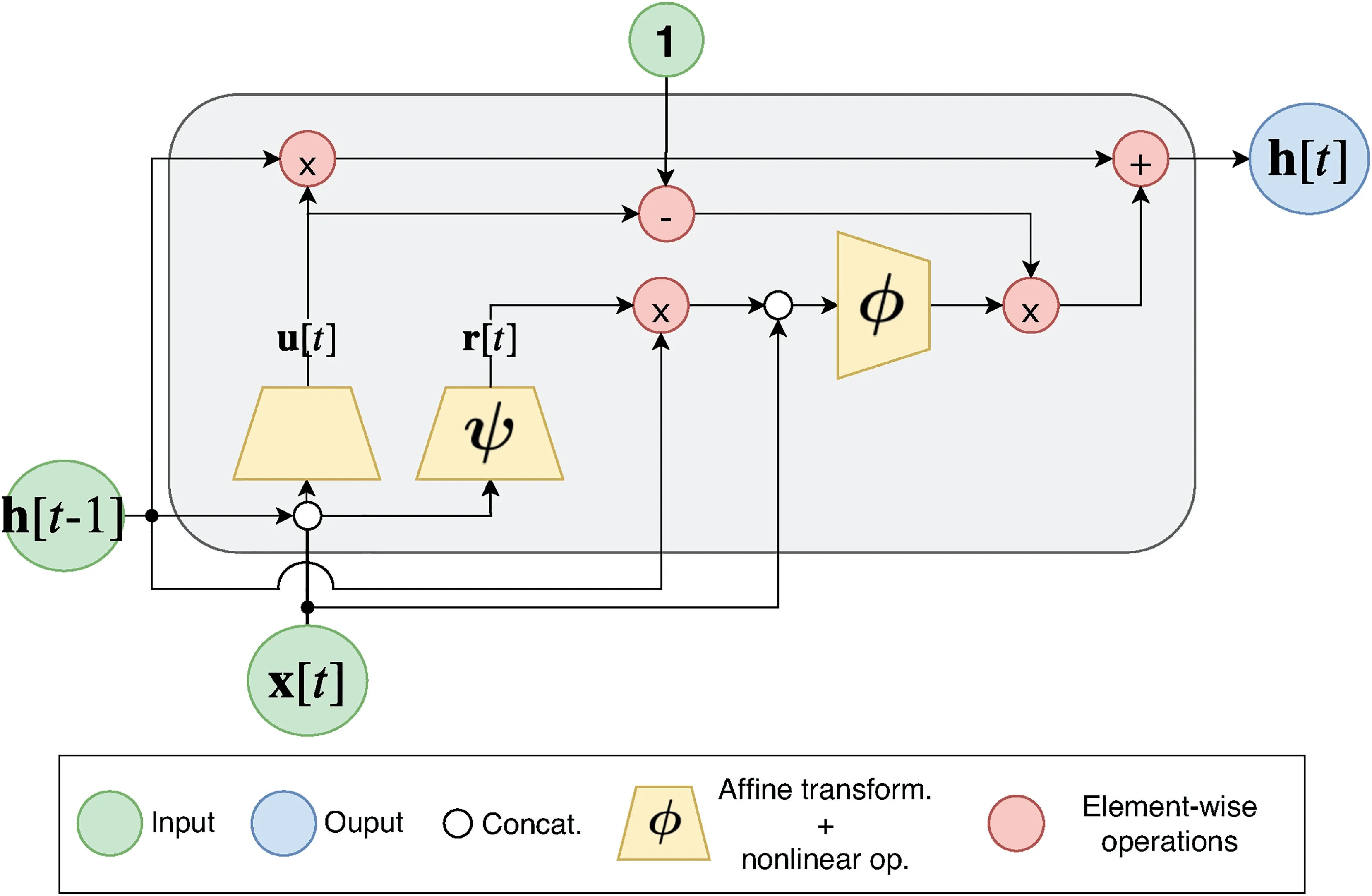
F I G U R E 5 Gated Recurrent Unit memory block with one cell
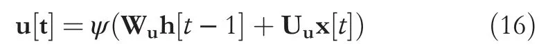

where Wu,Wr,Wc∈IRnH×nH, Uu,Ur,Uc∈IRnH×dare the parameters to be learnt,ψ(·) is generally a sigmoid activation,whileφ(·) can be any kind of non-linearity (in the original work it was a hyperbolic tangent).u[t] and r[t] are the update and reset gates, respectively.Several works in the natural language processing community show that GRUs perform comparably to LSTM but generally train faster due to their lighter computation [58, 59].
4.4|Deep recurrent neural networks
All recurrent architectures presented so far are characterised by a single layer.In turn, this implies that the computation is composed of an affine transformation followed by nonlinearity.That said, the concept of depth in RNN is less straightforward than in feedforward architectures.Indeed, the latter ones become deep when the input is processed by a large number of non-linear transformations before generating the output values.However, according to this definition, an unfolded RNN is already a deep model given its multiple nonlinear processing layers.That said, a deep multi-level processing can be applied to all the transition functions(input-hidden,hidden-hidden, and hidden-output) as there are no intermediate layers involved in these computations[60].Deepness can also be introduced in recurrent neural networks by stackingrecurrent layers one on top of the other [61].As this deep architecture is more intriguing, in this work, we refer to it as a Deep RNN.By iterating the RNN computation, the function implemented by the deep architecture can be represented as

where hℓ[t] is the hidden state at timesteptfor layerℓ.Notice that h0[t]=x[t].It has been empirically shown that Deep RNNs better capture the temporal hierarchy exhibited by time series then their shallow counterpart[60, 62, 63].Of course, hybrid architectures having different layers—recurrent or not—can be considered as well.
4.5|Multi-step prediction schemes
There are five different architecture-independent strategies for multi-step-ahead forecasting [64]:
4.5.1|Recursive strategy (Rec)
A single model is trained to perform a one-step-ahead forecast given the input sequence.Subsequently,during the operational phase, the forecasted output is recursively fed back and considered to be the correct one.By iterating this procedurenOtimes, we generate the forecast values at timet+nO.The procedure is described in Algorithm 1,where x[1:]is the input vector without its first element while thevectorize(·) procedure concatenates the scalar outputyto the exogenous input variables.

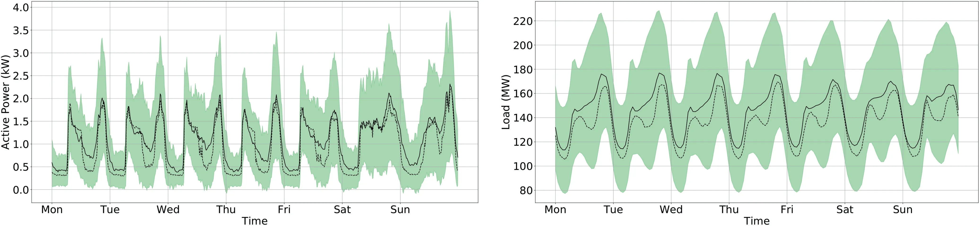
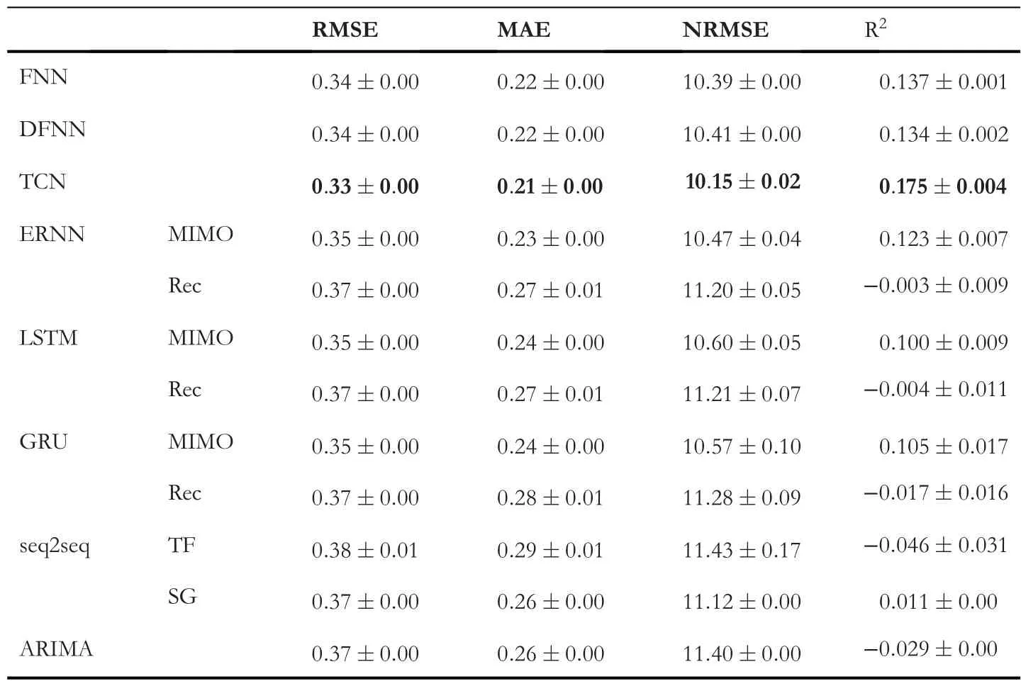
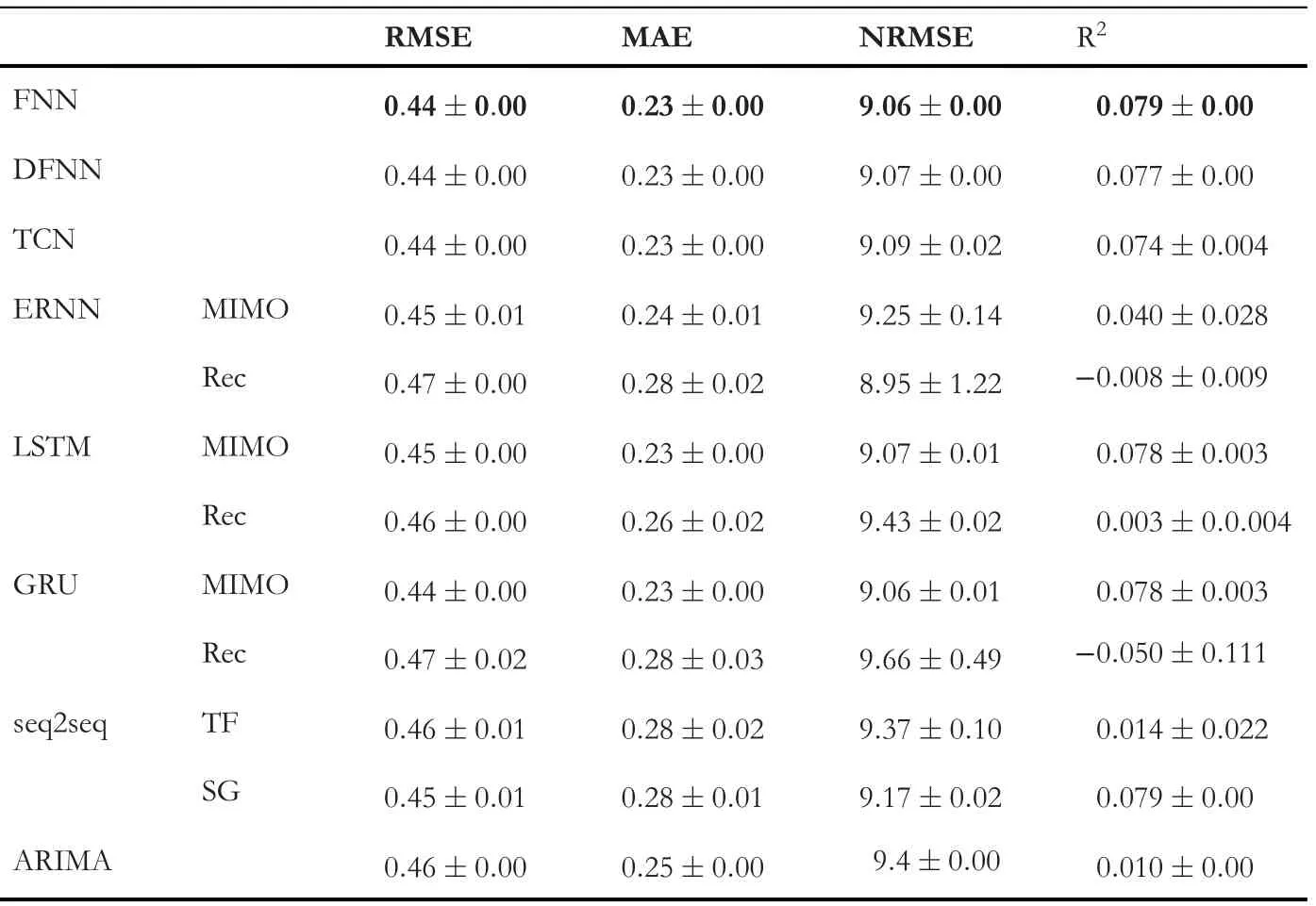
Algorithm 1 Recursive Strategy (Rec) for Multi-Step Forecasting 1: x ←x t: o ←empty li 2st 3: k ←1 4: while k To summarise,the predictorfreceives as input a vector x of lengthnTand outputs a scalar valueo. 4.5.2|Direct strategy Design a set ofnOindependent predictorsf k,k=1,…,nO,each of which provides a forecast at timet+k.Similar to the recursive strategy, each predictorfkoutputs a scalar valueo,but the input vector is the same for all the predictors.Algorithm 2 details the procedure. Algorithm 2 Direct Strategy for Multi-step Forecasting 1: x ←xt 2: o ←empty list 3: k ←1 4: while k 5: o ←concatenate(o,fk(x))6: k ←k+1 7: end while 8: return o as ^yt 4.5.3|DirRec strategy [65]is a combination of the above two strategies.Similar to the direct approach,nOmodels are used, but here, each predictor leverages on an enlarged input set, obtained by adding the results of the forecast at the previous timestep.The procedure is detailed in Algorithm 3. Algorithm 3 Direct Strategy for Multi-step Forecasting 1: x ←xt 2: o ←empty list 3: k ←1 4: while k 4.5.4|MIMO strategy Multiple input-Multiple output [66], a single predictorfis trained to forecast a whole output sequence of lengthnOin one shot,that is,different from the previous cases,the output of the model is not a scalar but a vector 4.5.5|DIRMO strategy [67], represents a trade-off between the direct strategy and the MIMO strategy.It divides thenOsteps forecasts into smaller forecasting problems, each of which is of lengths.It follows that 「」 predictors are used to solve the problem. Given the considerable computational demand required by RNNs during training, we focus on multi-step forecasting strategies that are computationally cheaper, specifically, recursive and MIMO strategies [64].We will call them RNN-Rec and RNN-MIMO. Given the hidden state h[t] at timestept, the hiddenoutput mapping is obtained through a fully connected layer on top of the recurrent neural network.The objective of this dense network is to learn the mapping between the last state of the recurrent network, which represents a kindof lossy summary of the task-relevant aspect of the input sequence and the output domain.This holds for all the presented recurrent networks and is consistent with Equation (9).In this work, RNN-Rec and RNN-MIMO differ in the cardinality of the output domain, which is 1 for the former andnOfor the latter, meaning that in Equation (9) either V ∈IRnH×1or V ∈IRnH×nO.The objective function is In [17], an Elmann recurrent neural network is considered to provide hourly load forecasts.The study also compares the performance of the network when additional weather information such as temperature and humidity are fed to the model.The authors conclude that, as expected, the recurrent network benefits from multi-input data and, in particular,weather ones.[28] makes use of ERNN to forecast household electric consumption obtained from a suburban area in the neighbouring areas of Palermo (Italy).In addition to the historical load measurements, the authors introduce several features to enhance the model's predictive capabilities.Besides the weather and the calendar information, a specific ad hoc index was created to assess the influence of the use of air conditioning equipment on the electricity demand.In recent years, LSTMs have been adopted in short-term load forecasting, proving to be more effective than traditional time series analysis methods.In [21], LSTM is shown to outperform traditional forecasting methods as it is able to exploit the long-term dependencies in the time series to forecast the day-ahead load consumption.Several studies proved to be successful in enhancing the recurrent neural network capabilities by employing multivariate input data.In[22], the authors propose a deep, LSTM-based architecture that uses past measurements of the whole household consumption along with some measurements from selected appliances to forecast the consumption of the subsequent time interval (i.e., a one-step prediction).In [23], a LSTM-based network is trained using a multivariate input, which includes temperature, holiday/working day information, and date and time information.Similarly, in [31], a power demand forecasting model based on LSTM shows an accuracy improvement compared to more traditional machine learning techniques such as gradient boosting trees and support vector regression. GRUs have not been used much in the literature as LSTM networks are often preferred.That said, the use of GRU-based networks is reported in [18], while a more recent study [24] uses GRUs for the daily consumption forecast of individual customers.Thus, investigating deep GRU-based architectures is a relevant scientific topic, also thanks to their faster convergence and simpler structure compared to LSTM [58]. Despite all these promising results, an extensive study of recurrent neural networks [18], and in particular of ERNN,LSTM, GRU, ESN [19] and NARX, concludes that none of the investigated recurrent architectures manages to outperform the others in all considered experiments.Moreover, the authors noticed that recurrent cells with gated mechanisms like LSTM and GRU perform comparably well than much simpler ERNN.This may indicate that in short-term load forecasting, the gating mechanism may be unnecessary; this issue is further investigated—and evidence found—in the present work. As a final comment, we observe that good results have been achieved in the past by using diversified computing architectures and hand-crafted features extracted from available data streams.Readers might then perceive this forecasting problem as solved and the exercise perform here purely academic.This is not true in several ways because (1) different computing architectures expose different approximation abilities.As such, for a given problem, one should test different non-linear families and identify the optimal one.(2)Huge data availability allows us to consider more complex—deep—architectures that can even tackle both fast and slow dynamics within the same model.The approximation error, i.e.,the discrepancy between the unknown dynamics describing the power consumption and those provided by the approximating one reduces.(3)From(2),it should be noted that even a very small (statistically sound) improvement in forecasting accuracy has a huge monetary and market impact—not to mention the sustainability asset.(4) Moreover, many dated papers suffer from inaccuracies in presenting the forecast performance as statistically sound assessments (e.g., K-fold cross-validation and statistical tests) have not been considered.(5) Finally, some deep learning architectures naturally learn in the first computational layers the best features solving the problem; this is an extra value that does not require any more handcraft feature design.That said, valuable handcraft features can always be taken into account and integrated with automatically extracted ones to further favour the inference performance. Sequence-to-sequence(seq2seq)architectures[68]or encoderdecoder models [51] were initially designed to solve RNNs'inability to produce output sequences of arbitrary length.The architecture was first used in neural machine translation[51,69,70]but has emerged as the golden standard in different fields such as speech recognition [62, 71, 72] and image captioning [73]. The core idea of this general framework is to employ two networks resulting in an encoder-decoder architecture.Thefirst neural network(possibly deep)f—the encoder—reads the input sequence xt∈IRnT×dof lengthnTone timestep at a time; the computation generates a, generally lossy, fixed dimensional vector representation of it c=f(xt,Θf),c ∈IRd'.This embedded representation is named context and can be the last hidden state of the encoder or a function of it.Then,a second neural networkg—the decoder—learns how to produce the output sequence ^yt∈IRnOgiven the context vector, that is, ^y=g(c,Θg).The schematics of the whole architecture is depicted in Figure 6. The encoder and the decoder modules are generally two recurrent neural networks trained together to minimise the objective function: This discrepancy between training and testing results in errors accumulating over time during inference.In the literature,this problem is often referred to as exposure bias[75].Several solutions have been proposed to address this problem;in[76],the authors present scheduled sampling, a curriculum learning strategy that gradually changes the training process by switching the decoder's inputs from ground-truth values to the model's predictions.Theprofessor forcingalgorithm,introduced in[77],uses an adversarial framework to encourage the dynamics of the recurrent network to be the same both at training and operational(test)time.Finally,in recent years,reinforcement learning methods have been adopted to train sequence-to-sequence models;a comprehensive review is presented in[78]. In this work, we investigate two sequence-to-sequence architectures,one trained viateacher forcing(TF)and one usingself-generated(SG) samples.The former is characterised by Equation (23) during training while Equation (24) is used during prediction.The latter architecture adopts Equation(24)both for training and prediction.The decoder's dynamics are summarised in Figure 7.It is clear that the two training procedures differ in the decoder's input source: ground-truth values in teacher forcing, estimated values in self-generated training. F I G U R E 6 seq2seq(Encoder-Decoder)architecture with a general Recurrent Neural network both for the encoder and the decoder networks.Assuming a Teacher Forcing training process,the solid lines in the decoder represent the training phase while the dotted lines depict the values path during prediction Only recently, seq2seq models have been adopted in shortterm load forecasting.In [33], a LSTM-based encoderdecoder model is shown to produce superior performance compared to the standard LSTM.In[79],the authors introduce an adaptation of RNN-based sequence-to-sequence architectures for time series forecasting of electrical loads to demonstrate its better performance with respect to a suite of models ranging from standard RNNs to classical time series techniques.The authors in[37]provide a similar empirical proof of the superior performance provided by sequence-to-sequence model when compared to standard deep neural network.Moreover, the study also suggests that using LSTM or GRU cells within the seq2seq architecture shell provides better results when compared against the Elmann unit.More recent studies in the field also consider an additional attention mechanism to the sequence-to-sequence model [38], which provides a more effective modelling of long-term temporal sequences while not requiring incredibly long input.The attention mechanism has been shown to provide good results in multi-step-ahead load forecasting both with univariate and multivariate time series [36]. Convolutional neural networks (CNNs) [80] are a family of neural networks designed to work with data that can be structured in a grid-like topology.CNNs were originally used on two-dimensional and three-dimensional images, but they are also suitable for one-dimensional data such as univariate time series.Once recognised as a very efficient solution for image recognition and classification [48, 81-83], CNNs have experienced wide adoption in many different computer vision tasks [84-88].Moreover, sequence modelling tasks, such as short-term electric load forecasting, have been mainly addressed with recurrent neural networks, but recent research indicates that convolutional networks can also attain state-ofthe-art performance in several applications including audio generation [89], machine translation [90] and time series prediction [91]. As the name suggests,these kind of networks are based on a discrete convolution operator that produces an output feature map f by sliding a kernel w over the input x. Each element in the output feature map is obtained by summing up the result of the element-wise multiplication between the input patch(i.e.,a slice of the input having the same dimensionality as the kernel) and the kernel.The number of kernels(filters)Mused in a convolutional layer determines the depth of the output volume(i.e.,the number of output feature maps).To control the other spatial dimensions of the output feature maps, two hyperparameters are used: stride and padding.Stride represents the distance between two consecutive input patches and can be defined for each direction ofmotion.Padding refers to the possibility of implicitly enlarging the inputs by adding (usually) zeros at the borders to control the output size.Indeed, without padding, the dimensionality of the output would be reduced after each convolutional layer. Considering a 1-D time series x ∈IRnTand a onedimensional kernel w ∈IRk, theithelement of the convolution between x and w is with f ∈IRnT-k+1if no zero-padding is used, otherwise the padding matches the input dimensionality, that is, f ∈IRnT.Equation (25)is referred to as the one-dimensional input case but can be easily extended to multi-dimensional inputs (e.g.,images, where x ∈IRW×H×D) [92].The reason behind the success of these networks can be summarised in the following four points: ●Local connectivity: each hidden neuron is connected to a subset of input neurons that are close to each other (according to a specific spatio-temporal metric).This property allows the network to drastically reduce the number of parameters to learn(with respect to a fully connected network)and facilitate computations. ●Parameter sharing: the weights used to compute the output neurons in a feature map are the same so that the same kernel is used for each location.This allows to reduce the number of parameters to learn. ●Translation equivariance: the network is robust to an eventual shifting of its input. ●Features free: these architectures free the designer from selecting and extracting handcraft features—a hard problem per se—as they are automatically extracted by the first learnt processing layers of the CNN. In our work, we focus on a convolutional architecture inspired by Wavenet [89], a fully probabilistic and autoregressive model used for generating raw audio waveforms and extended to time series prediction tasks [91]. To the best of the authors'knowledge,this architecture has never been proposed to forecast electric load.A recent empirical comparison between temporal convolutional networks and recurrent networks has been carried out in [93] on tasks such as polymorphic music and charter-sequence-level modelling.The authors were the first to use the name temporal convolutional networks(TCNs)to indicate convolutional networks that are autoregressive, able to process sequences of arbitrary length and output a sequence of the same length.To achieve the above, the network has to employ causal (dilated)convolutions, and residual connections should be used to handle a very long history size. Being TCNs, a family of autoregressive models, the estimated value at timetmust depend only on past samples and not on future ones (Figure 8).To achieve this behaviour in a convolutional neural network,the standard convolution operator is replaced by causal convolution.Moreover, zero-padding of length(filter size-1)is added to ensure that each layer has the same length of the input layer.To further enhance the network capabilities,dilated causal convolutions(DCCs) are used,allowing to increase the receptive field of the network(i.e.,the number of input neurons to which the filter is applied)and its ability to learn long-term dependencies in the time series (see Figure 9).Given a one-dimensional input x ∈IRnT, and a kernel w ∈IRk, a dilated convolution output using a dilation factordbecomes F I G U R E 7 (Left) decoder with ground-truth inputs (Teacher Forcing).(Right) Decoder with self-generated inputs This is a major advantage with respect to simple causal convolutions, as in the latter case the receptive fieldrgrows linearly with the depth of the networkr=k(L-1),while with dilated convolutions the dependence is exponentialr=2L-1k,ensuring that a much larger history size is used by the network. Despite the implementation of dilated convolution, the CNN still needs a large number of layers to learn the dynamics of the inputs.Moreover, the performance often degrades with the increase of the network depth.The degradation problem has been first addressed in [48], where the authors propose a deep residual learning framework.The authors observe that for aL-layers network with a training errorϵ, insertingkextra layers on top of it should either leave the error unchanged or improve it.Indeed, in the worst case scenario, the newkstacked non-linear layers should learn the identity mapping y=H(x)=x, where x is the output of the network havingLlayers and y is the output of the network withL+klayers.Although almost trivial, in practice, neural networks experience problems in learning this identity mapping.The proposed solution suggests that these stacked layers fit a residual mapping F(x)=H(x)-x instead of the desired one, H(x).The original mapping is recast into F(x)+x, which is realised by feed-forward neural networks with shortcut connections;in this way, the identity mapping is learnt by simply driving the weights of the stacked layers to zero. By means of the two aforementioned principles, the temporal convolutional network is able to exploit a large history size in an efficient manner.Indeed, as observed in[93], these models present several computational advantages compared to RNNs.In fact, they have lower memory requirements during training and the predictions for later timesteps are not done sequentially but can be computed in parallel exploiting parameter sharing.Moreover, TCNs'training is much more stable than that involving RNNs,allowing to avoid the exploding/vanishing gradient problem.For all of the above, TCNs have demonstrated to be a promising area of research for time series prediction problems, and here, we aim to assess their forecasting performance with respect to state-of-the-art models in short-term load forecasting.The architecture used in our work is depicted in Figure 10, which is, except for some minor modifications, the network structure detailed in [91].In the first layer of the network, we process separately the load information and, when available, the exogenous information such as temperature readings.Later, the results will be concatenated together and processed by a deep residual network withLlayers.Each layer consists of a residual block with 1-D DCC, a rectified linear unit (ReLU) activation and finally dropout to prevent overfitting.The output layer consists of 1 × 1 convolution, which allows the network to output a one-dimensional vector y ∈IRnThaving the same dimensionality as the input vector x.To approach multi-step forecasting, we adopt a MIMO strategy. In the short-term load forecasting relevant literature, CNNs have not been studied to a large extent.Indeed, until recently, these models were not considered for any time series-related problem.Still, several works tried to address the topic; in [15], a deep convolutional neural network model named DeepEnergy is presented.The proposed network is inspired by the first architectures used in ImageNet challenge (e.g.[81]), alternating convolutional and pooling layers, halving the width of the feature map after each step.According to the provided experimental results,DeepEnergy can precisely predict energy load in the next three days, outperforming five other machine learning algorithms including LSTM and FNN.In [16], a CNN iscompared to recurrent and feed-forward approaches,showing promising results on a benchmark dataset.In [25],a hybrid approach involving both convolutional and recurrent architectures is presented.The authors integrate different input sources and use convolutional layers to extract meaningful features from the historic load while the recurrent network's main task is to learn the system's dynamics.The model is evaluated on a large dataset containing hourly loads from a city in North China and is compared with a three-layer feed-forward neural network.A different hybrid approach is presented in [26]; the authors process the load information in parallel with a CNN and an LSTM.The features generated by the two networks are then used as an input for a final prediction network (fully connected) in charge of forecasting the day-ahead load.More recently, temporal convolutional networks have also started to be used and show very promising results indeed.In [39], a modified encoder-decoder architecture based on WaveNet is proposed.The authors performed careful testing of their model against the state-of-the-art power consumption data coming from the French grid.TCNs have been also used in probabilistic frameworks [40] to estimate probability densities in both parametric and nonparametric settings.The authors showed the superior performance of their method in both probabilistic forecasting and point estimates. F I G U R E 8 A three layers convolutional neural network with causal convolution (no dilation), the receptive field r is 4 F I G U R E 1 0 Temporal convolutional network Architecture.xt is the vector of historical loads along with the exogenous features for the time window indexes from 0 to nT, zt is the vector of exogenous variables related to the last nO indexes of the time window(when available),^yt is the output vector.Residual Blocks are composed by a 1D Dilated Causal Convolution, a ReLU activation and Dropout.The square box represents a concatenation between (transformed)exogenous features and (transformed) historical loads F I G U R E 9 A three layers convolutional neural network with dilated causal convolutions.The dilation factor d grows on each layer by a factor of two and the kernel size k is 2, thus the output neuron is influenced by eight input neurons, that is,, the history size is 8 In this section, we perform evaluation and assessment of all the presented architectures.The testing is carried out by means of five use cases that are based on three different datasets.As said in the introduction, our goal is to directly compare and assess relevant deep learning models on standardised publicly available benchmarks so as to fully support experiment reproducibility; also, the designed code is free and has been made available to researchers and practitioners.1https://github.com/albertogaspar/dts We first introduce the performance metrics that we considered for both network optimisation and testing, then describe the datasets that have been used and finally we discuss the results. The efficiency of the considered architectures has been measured and quantified using widely adopted error metrics.Specifically, we adopted the root mean squared error (RMSE)and the mean absolute error (MAE): whereNis the number of input-output pairs provided to the model in the course of testing,yi[t]and^yi[t],respectively,are the real load values and the estimated load values at timetfor samplei(i.e.thei-thtime window).〈·〉is the mean operator,‖·‖2is the Euclidean L2 norm,while‖·‖1is the L1 norm.y ∈IRnOand ^y ∈IRnOare the real load values and the estimated load values for one sample, respectively.Still, a more intuitive and indicative interpretation of the prediction efficiency of the estimators can be expressed by the normalised root mean squared error,which,different from the above two metrics,is independent from the scale of the data: whereymaxandyminare the maximum and minimum value of the training dataset, respectively.In order to quantify the proportion of variance in the target that is explained by the forecasting methods, we also consider the R2index: All considered models have been implemented in Keras 2.12 [94] with Tensorflow [95] as backend.The experiments are executed on a Linux cluster with an Intel(R)Xeon(R)Silver CPU and an Nvidia Titan XP. In this scenario,we aim at testing and validating the usability of the considered models in the case of inputs with very challenging and noisy dynamics.The first use case considers the individual household electric power consumption dataset(IHEPC), which contains 2.07 M measurements of electric power consumption for a single house located in Sceaux(7 km of Paris, France).Measurements are collected every minute between December 2006 and November 2010 (47 months)[29].In this study, we focus on predicting the ‘Global active power’parameter.Nearly 1.25%of measurements are missing,still, all the available ones come with timestamps.We reconstruct the missing values using the mean power consumption for the corresponding time slot across the different years of measurements.In order to have a unified approach, we have decided to resample the dataset using a sampling rate of 15 min, which is a widely adopted standard in modern smart metre technologies.In Table 3, the sample size is outlined for each dataset. In this use case, we performed the forecasting using only historical load values as relevant exogenous variables were not available.The right side of Figure 11 depicts the average weekly electric consumption.As expected, it can be observed that the highest consumption is registered in the morning and evening periods of the day when the occupancy of resident houses is high.Moreover, the average load profile over a week clearly shows that weekdays are similar while weekends present a different trend of consumption. The figure shows that the data are characterised by high variance.The prediction task consists in forecasting the electric load for the next day, that is, 96 timesteps ahead. In order to assess the performance of the architectures,we hold out a portion of the data that denotes our test setand comprises the last year of measurements.The remaining measurements are repeatedly divided in two sets, keeping aside a month of data every five months.This process allows us to build a training set and a validation set on which different hyperparameter configurations can be evaluated.Only the best performing configuration is later evaluated on the test set. The second and third use cases consider the data coming from the smart metring electricity customer behaviour trials (CBTs), which took place during 2009 and 2010 with over 5000 Irish homes and businesses participating[96].The data are collected and made available by the Commission for Energy Regulation (CER), which is the regulator for the electricity and natural gas sectors in Ireland.Since we are interested in evaluating the performance of our model on a single household, we selected 2 m(2113 and 4088) that, by showing a different consumption profile, become reference instances of the household class.In this way, reproducibility of results is granted; yet, some variability is considered.More household instances can be indeed considered but are outside the scope of this work.In this use case, as with the previous one, we performed the forecasting using only historical load values as no exogenous information is available.The forecasting horizon is still one day and the preprocessing method and the model selection criteria used are also the same.We report the average weekly electric consumption in Figure 12 for both considered metres.By looking at these images, we can immediately notice that both metres display high variance compared to use case I.In particular, metre 4088 presents a huge difference between its mean and median, which anticipates that prediction for this use case would be challenging. As the accurate consumption forecast of an area (e.g., supplied by a feeder, substation or even entire town) represents a very relevant problem in smart grids, in our assessment, we devote special attention to this scenario.We believe that the main contribution of our work to research and industry practice can actually be related to providing a clear insight into the usability of the proposed models to such issues.The other two use cases are based on the GEFCom2014 dataset[35], which was made available for an online forecasting competition that lasted between August 2015 and December 2015.The dataset contains 60.6k hourly measurements of(aggregated) electric power consumption collected by ISO New England between January 2005 and December 2011.Different from the dataset analysed before, temperature values are also available and are used by the different architectures to enhance their prediction performance.In particular, the input variables used for forecasting the subsequentnOat timesteptinclude several previous load measurements,the temperature measurements for the previous timesteps registered by 25 different stations, hour, day, month and yearof the measurements.We apply standard normalisation to load and temperature measurements while for other variables we simply apply one-hot encoding, that is, we code information inK-dimensional vector in which one of the elements equals 1, and all others equal 0 [97].On the right side of Figure 11, we observe the average load and data dispersion on a weekly basis.Compared to IHEPC and CERs, the load profiles here look much more regular.This meets intuitive expectations as the load measurements in the previous datasets come from a single household; thus, the randomness introduced by the user behaviour has a more remarkable impact on the results.On the contrary, the load information in GEFCom2014 comes from the aggregation of the data provided by several different smart metres; clustered data exhibits a more stable and regular pattern.The main task of these use cases, as well the previous one, consists in forecasting the electric load for the next day, that is, 24 timesteps ahead.The hyperparameters' optimisation and the final score for the models follow the same guidelines provided for use cases I, II and III; the number of points for each subset is described in Table 3. T A B L E 3 Sample size of training, validation and test sets for each dataset The compared architectures are the ones presented in the previous sections with one exception.In fact, we have additionally considered a deeper variant of a feed-forward neural network with residual connections, which is named DFNN in this work.In accordance with [98], we have employed a 2-shortcut network, that is, the input undergoes two affine transformations each followed by a non-linearity before being summed to the original values.For regularisation purposes, we have included dropout and batch normalisation [99] in each residual block.We have additionally inserted this model in the results' comparison as it represents an evolution of standard feed-forward neural networks,which is expected to better handle highly complex time series data. F I G U R E 1 2 Weekly statistics for the electric load reported by smart metres 2113 (right) and 4088 (left) in the commission for energy regulation dataset.The bold line is the mean curve, the dotted line is the median and the green area covers one standard deviation from the mean F I G U R E 1 1 Weekly statistics for the electric load in the whole IHEPC (Left) and GEFCom2014 datasets (right).The bold line is the mean curve, the dotted line is the median and the green area covers one standard deviation from the mean Moreover, to allow comparison between deep learning models and standard time series analysis technique, we additionally consider an ARIMA model in the experimental evaluation (AR, ARMA or ARMAX models are not worth considering here as none of the considered time series is stationary). Table 4 summarises the best configurations found through grid search for each model and use case.For all datasets, we experimented different input sequences of lengthnT.Finally, we used a window size of four days,which has been found to be the best trade-off between performance and memory requirements.The output sequence lengthnOis fixed to one day.For each model,we identified the optimal number of stacked layers in the networkL, the number of hidden units per layernH, the regularisation coefficientλ(L2 regularisation) and the dropout ratepd.Moreover, for TCN, we additionally tuned the widthkof the convolutional kernel and the number of filters applied at each layerM(i.e., the depth of each output volume after the convolution operation).The dilation factor is increased exponentially with the depth of the network, that is,d=2ℓwithℓbeing theℓ-thlayer of the network. Tables 5 to 7 summarise the test scores of the presented architectures obtained for the IHEPC dataset, the CER dataset with metre id 2113 and the one with metre id 4088, respectively.Certain similarities among networks trained for different use cases can be spotted out already at this stage.In particular, we observe that all models exploit a small number of neurons.This is not usual in deep learning but—at least for recurrent architectures—is consistent with [18]. Among recurrent neural networks, we observe that, in general, the MIMO strategy outperforms the recursive one in this multi-step prediction task.This is reasonable in the individual household scenario.Indeed, the recursive strategy,different from the MIMO one, is highly sensitive to error accumulation,which,in a highly volatile time series as the ones addressed here, results in a very inaccurate forecast.Among the MIMO models, we observe that in some cases (see Table 5)gated networks perform slightly better than the simple Elmann network,but this is not a common pattern among the investigated datasets.Thus, for customer-level load forecasting, there is no sufficient evidence to claim the superiority of gated systems.In general, we notice that all models, except the RNNs trained with a recursive strategy, achieve comparable performance and none really stands out.It is interesting to comment that recurrent networks outperform sequence-tosequence architectures, which are supposed to better model complex temporal dynamics like the one exhibited by the residential load curve.Nevertheless, by observing the performance of recurrent networks trained with the recursive strategy, this behaviour is less surprising.In fact, compared with the aggregated load profiles, the load curve belonging to a single smart metre is way more volatile and sensitive to customer behaviour.For this reason, leveraging geographical and socio-economic features that characterise the area where the user lives may allow deep networks to generate better predictions.The statement above is valid for the IHEPC dataset and CER - 2113, while for CER - 4088 the described behaviours are less evident.This comes from the last use case being dominated by noise, and as such, being hardly predictable.On the contrary, metre 2113 and IHEPC have more predictable patterns and indeed,by looking at the results tablesone can immediately notice how models' performance are distributed on a much wider range.For use cases I and II a classical method like ARIMA is easily outperformed by all considered deep learning techniques.Once again, this is not true for use case III for reasons explained above.For visualisation purposes, we compare all the models' performance for IHEPC.On the left side of Figure 13, we outline a single-day prediction scenario while on the right side of Figure 13, we quantify the differences between the best predictor(the GRUMIMO)and the actual measurements;the thinner the line,the closer the prediction to the true data.Furthermore, in this figure,we concatenate multiple day predictions to have a wider time span and evaluate the model predictive capabilities.We observe that the model is able to generate a prediction that correctly models the general trend of the load curve but fails to predict steep peaks.This might come from the design choice of using MSE as the optimisation metric, which could discourage deep models from predicting high peaks as large errors are hugely penalised, and therefore, predicting a lower and smoother function results in better performance according to this metric.Alternatively, some of the peaks may simply represent noise due to a particular user behaviour and are thus unpredictable by definition. T A B L E 4 Best configurations found via grid search for all dataset used The load curve of the second dataset (GEFCom2014)results from the aggregation of several different load profiles producing a smoother load curve when compared with the individual load case.Hyperparameters' optimisation and the final score for the models can be found in Table 4. Table 8 and Table 9 show the experimental results obtained by the models in two different scenarios.In the former case,only load values were provided to the models while in the latter scenario the input vector has been augmented with the exogenous features described before.Compared to the previous dataset, this time series exhibits a much more regular pattern;as such we expect the prediction task to be easier.Indeed, we can observe a major improvement in terms of performance across all the models. T A B L E 5 Individual household electric power consumption dataset results T A B L E 6 CER results (metre 2113) As already noted in [22, 100], the prediction accuracy increases significantly when the forecasting task is carried out on a smooth load curve (resulting from the aggregation of many individual consumers). We can observe that,in general,all models except ARIMA and plain FNNs benefit from the presence of exogenous variables.When exogenous variables are adopted, we notice amajor improvement by RNNs trained with the recursive strategy, which outperform MIMO ones.This increase in accuracy can be attributed to a better capacity of leveraging the exogenous time series of temperatures to yield a better load forecast.Moreover, RNNs with the MIMO strategy gain negligible improvement compared to their performance when no extra feature is provided.This kind of architectures use a feed-forward neural network to map their final hidden state to a sequence ofnOvalues, that is, the estimates.Exogenous variables are elaborated directly by this FNN, which, as observed above,have problems in handling both load data and extra information.Consequently, a better way of injecting exogenous variables in the MIMO recurrent network needs to be found in order to provide a boost in prediction performance comparable to the one achieved by employing the recursive strategy. F I G U R E 1 3 (Right) Predictive performance of all the models on a single day for IHEPC dataset.The left portion of the image shows (part of) the measurements used as input while the right side with multiple lines represents the different predictions.(Left)Difference between the best model's predictions(gated recurrent units-multiple input-multiple output) and the actual measurements.The thinner the line the closer the prediction is to the true data T A B L E 7 CER results (metre 4088) For reasons that are similar to those discussed above,sequence-to-sequence models trained viateacher forcing(seq2seq-TF) experienced improvement when exogenous features were used.Still, seq2seq models trained in the freerunning mode (seq2seq-SG) proves to be a valid alternative to standard seq2seq-TF producing high quality predictions in all use cases.The absence of a discrepancy between training and inference in terms of data generating distribution shows to be an advantage as seq2seq-SG is less sensitive to noise and error propagation. Finally, we notice that TCNs perform well in all the presented use cases.Considering their lower memoryrequirements in the training process along with their inherent parallelism, this type of networks represents a promising alternative to recurrent neural networks for short-term load forecasting. T A B L E 8 GEFCom2014 results without any exogenous variable.Each model's mean score(±one standard deviation)comes from 10 repeated training processes T A B L E 9 GEFCom2014 results with exogenous variables As a final note, we can observe that the ARIMA model is outperformed by all other approaches.This confirms that,also for aggregated load consumption, deep learning approaches are much more effective than classical techniques due to the presence of non-linearities. The prediction results are presented in the same fashion as the previous use case in Figure 14.Observe that, in general, all considered models are able to produce reasonable estimates as sudden picks in consumption are smoothed.Therefore, predictors greatly improve theiraccuracy when predicting day-ahead values for the aggregated load curves with respect to an individual household scenario. F I G U R E 1 4 (Right)Predictive performance of all the models on a single day for GEFCom2014 dataset.The left portion of the image shows(part of)the measurements used as input while the right side with multiple lines represents the different predictions.(Left)Difference between the best model's predictions(long short-term memory-Rec) and the actual measurements.The thinner the line the closer the prediction to the true data In this work, we have surveyed and experimentally evaluated the most relevant deep learning models applied to the short-term load forecasting problem, paving the way for standardised assessment and identification of the most optimal solutions in this field.The focus has been given to the three main families of models, namely, recurrent neural networks, sequence-to-sequence architectures and recently developed temporal convolutional neural networks.An architectural description along with a technical discussion on how multi-step ahead forecasting is achieved, has been provided for each considered model.Moreover, different forecasting strategies are discussed and evaluated, identifying advantages and drawbacks for each of them.The evaluation has been carried out on five real-world use cases that refer to two distinct scenarios for load forecasting.Indeed, three use cases deal with datasets coming from a single household characterised by noisy dynamics while the other two tackle the prediction of a load curve that represents aggregated metres, dispersed over a wide area of the grid.Our findings concerning the application of recurrent neural networks to short-term load forecasting, show that the simple ERNN performs comparably to gated networks such as GRU and LSTM when adopted in aggregated load forecasting.Thus, the less costly alternative provided by ERNN may represent the most effective solution in this scenario as it allows to reduce the training time without remarkable impact on prediction accuracy.A similar conclusion may be drawn for a single-household electric load forecasting, where only in one use case gated networks prove to be superior to Elmann ones.Sequence-tosequence models have demonstrated to be quite efficient in load forecasting tasks even though they seem to fail in outperforming RNNs.In general, we can claim that seq2-seq architectures do not represent a golden standard in load forecasting as they do in other domains such as natural language processing.In addition, regarding this family of architectures, we have observed that teacher forcing may not represent the best solution for training seq2seq models on short-term load forecasting tasks.Despite being harder in terms of convergence, free-running models learn to handle their own errors, avoiding the discrepancy between training and testing that is a wellknown issue for teacher forcing.It turns out to be worth the effort to further investigate the capabilities of seq2seq models trained with intermediate solutions such asprofessor forcing.Finally, we evaluated the recently developed temporal convolutional neural networks, which demonstrated convincing performance when applied to load forecasting tasks.Therefore, we strongly believe that the adoption of these networks for sequence modelling in the considered field is very promising (especially for aggregated loads) and might even introduce a significant advance in this area that is emerging as important for future smart grid development.We also comment that short-term load forecasting at the customer level has proved to be an extremely challenging task for deep learning models as well.As a future direction in this specific topic, we are interested in exploiting time series correlation to learn a single model for multiple metres that exhibits similar behaviour.Our preliminary results are promising [101] and we believe that such an approach may provide considerable improvement in the field compared to the approach presented here.We hope that the presented work as well as the open sourcing of a library for short-term load forecasting may stimulate other authors to contribute to the research in the field. ACKNOWLEDGEMENTS This project is carried out within the frame of the Swiss Centre for Competence in Energy Research on the Future Swiss Electrical Infrastructure (SCCER-FURIES) with the financialsupport of the Swiss Innovation Agency(Innosuisse-SCCER program). DATA AVAILABILITY STATEMENT The data that support the findings of this study are derived from the following resources available in the public domain: https://archive.ics.uci.edu/ml/datasets/individual+household+electric+power+consumption, http://blog.drhongtao.com/2017/03/gefcom2014-load-forecasting-data.html, https://www.ucd.ie/issda/data/commissionforenergyr egulationcer/.Restrictions apply to the availability of these data, which were used under licence for this study. ORCID Alberto Gasparinhttps://orcid.org/0000-0003-3350-3168


4.6|RNNs' application for short-term load forecasting
5|SEQUENCE-TO-SEQUENCE MODELS


5.1|seq2seq application for short-term load forecasting
6|CONVOLUTIONAL NEURAL NETWORKS

6.1|Dilated causal convolution


6.2|Residual connections
6.3|CNNs and TCNs' application for short-term load forecasting

7|PERFORMANCE ASSESSMENT


7.1|Performance metrics


7.2|Use case I, II and III (individual households)
7.3|Use cases IV and V (aggregated load)

7.4|Results


8|CONCLUSIONS
杂志排行

CAAI Transactions on Intelligence Technology的其它文章
- Head-related transfer function-reserved time-frequency masking for robust binaural sound source localization
- A hierarchical optimisation framework for pigmented lesion diagnosis
- A spatial attentive and temporal dilated (SATD) GCN for skeleton-based action recognition
- Improving data hiding within colour images using hue component of HSV colour space
- Several rough set models in quotient space
- Shoulder girdle recognition using electrophysiological and low frequency anatomical contraction signals for prosthesis control