Research progress on seismic imaging technology

Zhen-Chun Li ,Ying-Ming Qu ,*

a School of Geosciences,China University of Petroleum,Qingdao,Shandong,266580,China

b Shandong Provincial Key Laboratory of Deep Oil & Gas,China University of Petroleum,Qingdao,Shandong,266580,China

Keywords:Common reflection surface stack Gaussian-beam migration Reverse-time migration Least-squares reverse-time migration

ABSTRACT High-precision seismic imaging is the core task of seismic exploration,guaranteeing the accuracy of geophysical and geological interpretation.With the development of seismic exploration,the targets become more and more complex.Imaging on complex media such as subsalt,small-scale,steeply dipping and surface topography structures brings a great challenge to imaging techniques.Therefore,the seismic imaging methods range from stacking-to migration-to inversion-based imaging,and the imaging accuracy is becoming increasingly high.This review paper includes:summarizing the development of the seismic imaging;overviewing the principles of three typical imaging methods,including common reflection surface (CRS) stack,migration-based Gaussian-beam migration (GBM) and reverse-time migration (RTM),and inversion-based least-squares reverse-time migration (LSRTM);analyzing the imaging capability of GBM,RTM and LSRTM to the special structures on three typical models and a land data set;outlooking the future perspectives of imaging methods.The main challenge of seismic imaging is to produce high-precision images for low-quality data,extremely deep reservoirs,and dual-complex structures.

1.Introduction

Seismic imaging technology contains three categories:stacking-,migration-and inversion-based imaging.Stacking imaging methods mainly include the common middle point(CMP)stack,the common reflection point (CRP) stack,the common conversion point (CCP)stack,and the common reflection surface (CRS,Hubral,1983;Tygel et al.,1996;Hubral et al.,1996) stack.Some field data examples suggest that the CRS stack is better than the other stacking-based imaging methods in low coverage and low signal-to-noise ratio(SNR) data.After conducting the CRS stack,a high-resolution zerooffset (ZO) profile and key kinematic parameters of the seismic wavefield can be obtained to directly invert the optimal velocity models.In the case of low SNR data,accurate kinematic parameters obtained from the CRS stack can help to produce a good initial model for the other velocity inversion methods.However,stacking-based imaging methods cannot accurately move dipping reflectors into their true subsurface positions and collapses diffractions.

Migration-based imaging is an effective technique for imaging complex structures (O'Brien and Gray,1996;Rosenberg,2000;Glogovsky et al.,2002;Ravasi and Curtis,2013).Up to now,prestack depth migration has become the mainstream in seismic exploration due to its high imaging accuracy.There are two main types of prestack depth migration methods.The first is based on the ray theory,such as Kirchhoff migration(Schneider,1978;Kuo and Dai,1984;Dai and Kuo,1986;Wapenaar and Haime,1990;Hokstad,2000;Wu et al.,2007b;Du and Hou,2008) and Gaussian-beam migration (GBM) (Hill,1990,2001;Alkhalifah,1995;Gray and Bleistein,2009;Yang et al.,2015a,2015b).The second method is wave-equation-based migration,such as one-way wave-equation migration(Gazdag,1978;Stolt,1978;Gazdag and Sguazzero,1984;Stoffa et al.,1990;Ristow and Rühl,1994;Mulder and Plessix,2004)and reverse-time migration (RTM) based on the two-way wave equation (Whitmore,1983;McMechan,1983;Baysal et al.,1983;Loewenthal and Mufti,1983;Sun and McMechan,1986).Among the ray-based migration methods,GBM has attracted more attention because Gassian-beams presents seismic wave fields more accurate than other geometric rays.RTM has advantages over one-way wave-equation migration methods for imaging complex subsurface structures.Therefore,the rest of the paper focuses on the raybased GBM and the two-way wave-equation-based RTM.

In the early 1980s,Cerveny et al.(1982)introduce the GBM from electromagnetism to geophysics.At first,it is used in the seismic wave forward modeling,and then gradually extended to the migration imaging (Hill,1990).Hill (2001) derive the poststack depth migration formula based on the Green function of Gaussian beam,which lays the theoretical basis for GBM.Subsequently,many geophysicists have improved the GBM to have a better adaptability and higher imaging accuracy(e.g.Nowack et al.,2003;Gray,2005).RTM can produce an image of the subsurface reflector by synthesizing forward-propagated source wavefields and backpropagated receiver wavefields,proposed by Whitmore (1983),McMechan (1983),Baysal et al.(1983) and Loewenthal and Mufti(1983).It exhibits a great advantage over ray-based methods and one-way wave-equation-based methods in imaging complex structure models(Chang and McMechan,1986,1990).Initially,RTM is implemented for post-stack migration.Chang and McMechan(1986) first applied RTM to prestack data processing.Due to the expensive computational cost of RTM,it has not been widely used in the industrial industry at first.But with the development of computer hardware,RTM starts to attract more attention from scholars and the industry.At present,RTM has moved from poststack to prestack (Chang and McMechan,1986),from 2D to 3D(Chang and McMechan,1990;Sun and McMechan,2001;Sun et al.,2006),from acoustic waves to elastic waves (Sun and McMechan,1986;Zhe and Greenhalgh,1997;Sun et al.,2006;Yan and Sava,2008;Qu et al.2015,2018;Zou et al.,2020),from isotropic media to anisotropic media (Liu et al.,2009;Huang et al.,2009;Tessmer,2010).As of now,RTM is the most accurate and robust depth migration method among all these methods (Baysal et al.,1983;McMechan,1983) because it does not make any approximation to the wave equation,and makes full use of the kinematics and dynamics information of the wave equation.It can deal with all wave types (reflection,refraction and diffraction) and has no imaging inclination limit (Chattopadhyay and McMechan,2008).The amplitude characteristics of the imaging results are maintained well(Mulder and Plessix,2004).

Most conventional migration methods use the adjoint of the forward operator rather than its inverse (Claerbout and Abma,1992;Nemeth et al.,1999),leading to a series of imaging problems,such as low SNR,unbalanced imaging amplitude and acquisition footprint,etc.(Kuehl and Sacchi,1999;Duquet et al.,2000).To overcome the problems of the conventional migration methods,least-squares migration (LSM) based on the adjoint state theory have been proposed and developed rapidly.Since the construction of the seismic inversion framework,the LSM is implemented within ray-based(e.g.Tarantola,1984;Cole and Karrenbach,1992;Duquet et al.,2000;Yue et al.,2021),one-way wave-equationbased (e.g.Kuehl and Sacchi,2001,2003;Rickett,2003) and twoway wave-equation-based (e.g.Zhang et al.,2015;Sun et al.,2018) migration operators.The ray-based LSM can be divided into least-squares Kirchhoff migration (LSKM) (e.g.Cole and Karrenbach,1992;Nemeth et al.,1999;Duquet et al.,2000;Fomel et al.,2002;Huang et al.,2013;Liu et al.,2013;Wang et al.,2014)and least-squares Gaussian-beam migration(LSGBM)(e.g.Hu et al.,2016a;Yuan et al.,2017;Yang et al.,2018;Yue et al.,2021).The oneway wave-equation-based LSM mainly includes least-squares splitstep Fourier migration(Kuehl and Sacchi,2001,2003;Shen and Liu,2012),least-squares generalized screen migration (Wu and Maarten,1996;Zhou et al.,2014),least-squares Fourier finitedifference migration (Rickett,2003;Yang and Zhang,2008),etc.Two-way wave-equation-based LSM is also known as least-squares RTM (LSRTM),which has drawn wide attention and research because of its advantage in imaging complex structures.To improve the effectiveness of LSRTM for migrating the field data,many optimization methods have been proposed to improve the computational efficiency(e.g.Plessix and Mulder,2004;Valenciano et al.,2006;Schuster et al.,2011;Huang and Schuster,2012;Dai et al.,2013;Wu et al.,2016;Chen and Sacchi,2017),reduce the dependence on the migration velocity (e.g.Hou and Symes,2016;Sun et al.,2018),suppress the effects of the seismic wavelets (e.g.Choi and Alkhalifah,2011)and mitigate the sensitivity to noise(e.g.Brossier et al.,2010;Aravkin et al.,2011).

This paper firstly reviews stacking-based CRS stack,migrationbased GBM and RTM,and inversion-based LSRTM.Then,several typical models and field data are tested by using GBM,RTM,and LSRTM separately.Finally,the future development of seismic imaging is prospected.

2.Imaging methods

2.1.Stacking-based CRS stack

The idea of CRS stack first comes from Hubral (1983).He first proposed the stacking method of common reflection element(CRE)based on two-parameters optimization(Keydar et al.,1989;Olalde and Rabbel,1995;Steentoft and Rabbel,1992,1994;Steentoft,1993)and CRS based on three-parameters optimization (Muller et al.,1998;Bazelaire et al.,1999;Oliva et al.,2010).Fig.1a,b and 1c show schematic diagram of MZO,Kirchhoff Prestack depth migration (PSDM) and CRS stack(Hubral et al.,1996).

In the coordinate system established by the middle pointxmand half offseth,the approximate formula of hyperbolic travel time on the CRS surface is

and the approximate formula of parabolic travel time on the CRS surface is

wherev0is the near-surface velocity,α is the emergence angle of ZO rays on the surface,RNIPis the curvature radius of the normal incident point wave front andRNis the curvature radius of the normal wave front.

Fig.2 shows CMP and CRS stacking images using a field data set.As can be seen from the comparison in Fig.2,the SNR of the CRS stacking profile is greatly improved,and the kinematic characteristics of the wavefield are maintained well.In particular,the image of deep reflectors is greatly enhanced.

2.2.Gaussian-beam migration and reverse-time migration

2.2.1.Gaussian-beam migration

The most critical step in GBM is to construct the Green function.In fact,the Green function can be understood as the seismic wavefield generated by a point source,which can be solved by the following equation

Fig.1.Schematic diagram of MZO (a),Kirchhoff PSDM (b) and CRS stack (c).

whereGGB（x，x0;ω）denotes the Green function,x is the coordinate,x0is the source point coordinate,v presents the velocity and ∇2denotes the Laplacian operator.

As the seismic exploration pursues higher and higher accuracy,the conventional GBM cannot meet the requirements of high precision imaging,so many new GBM methods and optimization algorithms have emerged,including the Gaussian beam reverse time migration (GBRTM) (Popov et al.,2010;Yang et al.,2015b;Zhang et al.,2019),elastic GBM (Huang et al.,2017),the true amplitude GBM(Albertin et al.,2004;Gray and Bleistein,2009),Fresnel-bandbased GBM(Yang and Zhu,2018),the least-squares Gaussian beam migration (LSGBM) (Hu et al.,2016a;Yuan et al.,2017;Yang et al.,2018),anisotropic GBM (Alkhalifah,1998),viscoacoustic GBM (e.g.Wu et al.,2015;Bai et al.,2016;Dai et al.,2016),etc.

In addition,other seismic beam migration methods,such as Fresnel beam and focusing beam(as shown in Figs.3 and 4),show better effects on seismic imaging of complex media and thus have been widely used.

2.2.2.Reverse time migration

The theoretical basis of RTM imaging is the time consistency principle proposed by Claerbout (1971).The imaging condition in the frequency domain can be expressed by the following equation

whereRrepresents the imaging result,Udenotes the receiver wavefield (the upgoing wavefield),ω denotes the frequency,Dis the source wavefield(the downgoing wavefield),(x,y,z)represents the spatial coordinates,sdenotes the source andtrepresents the time.In some frequencies,Din equation (4) will be very small,or even zero,which leads to instability of the imaging condition.For this reason,Claerbout(1971)approximated equation(4)to produce the imaging result by using a zero-delay cross-correlation of upgoing and downgoing waves,which can be expressed as

wheresmaxandtmaxrepresent the maximum shot number and the maximum recording time,respectively.

The imaging condition expressed in equation(5)can also apply to RTM.As a result,RTM includes three steps:(1) the forward continuation of the source-side wavefield,(2) the backward continuation of the receiver-side wavefield and(3)the application of imaging conditions (Chang and McMechan,1986).

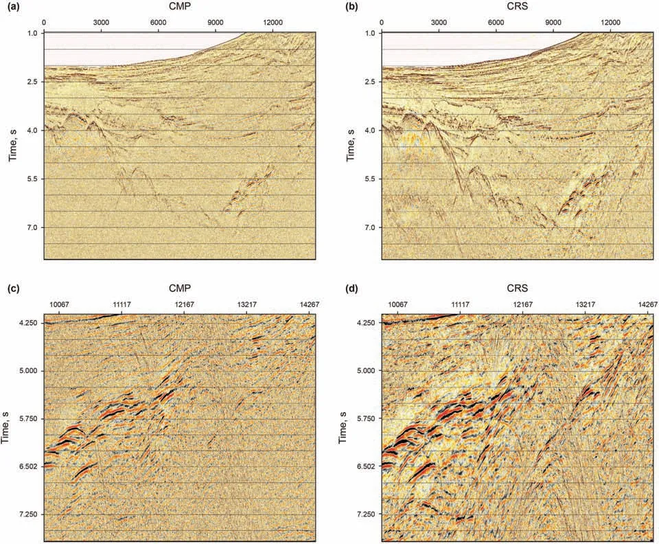
Fig.2.CMP (a) and CRS (b) stacking profiles and magnified views in Fig.2a (c) and 2b (d).

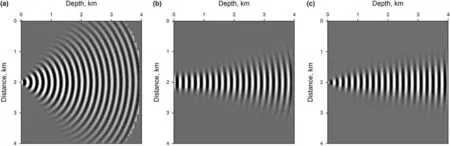
Fig.3.Propagation morphology of GB and Fresnel beam.(a) GB with an initial width of 1/4 wavelength;(b) GB with an initial width of one wavelength;(c) Fresnel beam.

A great deal of research has been done on several defects of RTM.There are two main methods to improve computational efficiency and storage capacity.One is to use high-performance computation (e.g.Foltinek et al.,2009;He et al.,2010;Suh et al.,2010;Liu et al.,2010;Zhao,2021),and the other is to improve algorithms (Hayashi and Burns,1999;Symes,2007;Zhang et al.,2007b;Dussaud and Symes,2008;Guan et al.,2008;Clapp,2009;Xu et al.,2010;Nguyen and McMechan,2013).

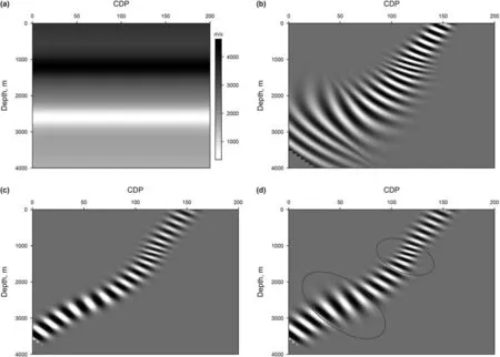
Fig.4.A velocity model (a) and propagation patterns of GB (b),dynamic focusing beam (c) and adaptive focusing beam (d).

Eliminating both low-wavenumber and high-wavenumber artifacts of migration is also a huge challenge in RTM.The proposed methods for this purpose includes three main categories:the first is to change the wave equation to attenuate the artifacts during in the stage of wave propagation(e.g.Baysal et al.,1984;Loewenthal et al.,1987;Fletcher et al.,2005);the second is to improve the imaging conditions by using the Poynting vector (e.g.Yoon and Marfurt,2006) and decomposing wavefields into up-going and down-going ones (Liu et al.,2011a),etc;the third is to apply post-imaging filtering,such as Laplacian filtering,least-squares filtering (Guitton et al.,2007),dip filtering(Sun and Zhang,2009),etc.

2.3.Inversion-based least-squares reverse time migration imaging

The purpose of LSM is to seek a model by minimizing an objective function.The common used objective function is based on the L2 norm and the objective functionEis given as

whereLrepresents a demigration operator(linear modeling operator),mdenotes the parameters,dobsrepresents the observed data set and ‖‖2denotes theL2-norm andmis a reflectivity model.

In recent years,the research of LSRTM mainly focuses on improving computational efficiency.The first method to improve efficiency is multisource LSRTM.Multisource LSRTM technology can combine a bunch of shot gathers into one or more supergathers for imaging,but crosstalk noise will be introduced.Some encoding technologies such as polarity encoding (e.g.Schuster et al.,2011),amplitude encoding (e.g.Hu et al.,2016b),frequency division encoding (e.g.Huang and Schuster,2012),plane wave encoding(e.g.Dai and Schuster,2013),random encoding(Li et al.,2018)and other encoding methods of LSRTM have been proposed to suppress the crosstalk noise.The second method is LSRTM based on gradient preprocessing.The method can improve the convergence rate by considering the inverse of the Hessian matrix as a preconditioner.However,solving the inverse of Hessian matrix needs a huge amount of computational cost,therefore,simplified Hessian matrices are introduced to preprocess gradients (e.g.Plessix and Mulder,2004;Valenciano et al.,2006;Gao et al.,2020).The third method is LSRTM based on regularization constraints.Reasonable regularization constraints can improve the convergence speed of LSRTM (Dai et al.,2013;Li et al.,2017a).The regularization constraint methods mainly include the local inclination constraint method (Liu et al.,2013),the prior information constraint method(Li et al.,2016),L1 sparse constraint(Wu et al.,2016,2021),sparse constraint in curved wave domain (Gao et al.,2020),local Radon transform constraint (Dutta et al.,2017),constraint in wavelet transform domain (Li et al.,2020a),etc.In addition,some instructive studies of practical LSRTM are implemented to reduce the dependence on the migration velocity (e.g.Liu and Li,2015;Hou and Symes,2016;Li et al.,2017c;Sun et al.,2018;Yang et al.,2020),the dependence on wavelets (e.g.Choi and Alkhalifah,2011;Li et al.,2017b),and the sensitivity to noise (e.g.Brossier et al.,2010;Aravkin et al.,2011;Li et al.,2017b).

3.Case study

3.1.Typical model examples

Some representative complex models are selected to numerical analyze the imaging capability of GBM,RTM and LSRTM to the special structures such as salt domes,small-scale anomalies and steeply dipping reflectors.

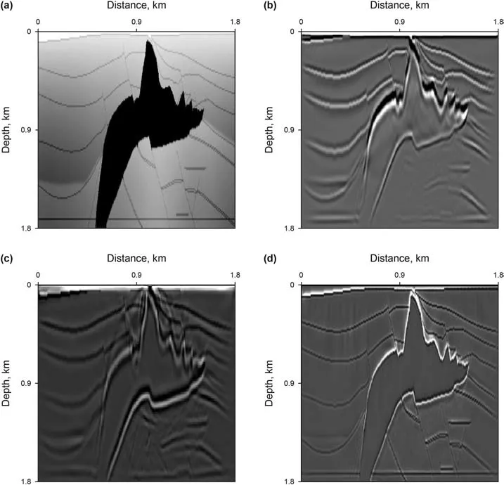
Fig.5.The salt dome model (a) and the imaging results from GB (b),RTM (c) and LSRTM (d).

3.1.1.Salt dome model

Firstly,a salt dome model is used to compare the three imaging methods on imaging the salt dome and subsalt structures.Fig.5a shows the saltdomevelocity modelwithagridsizeof301×301anda grid interval of 6 m.The model spans a rectangle area of 4800 m×3200 m and has a saltdomewithsteeply dipping flanks and subsalt structures,bringing a great challenge for imaging.The shot record consists of 75 shots,each with 301 traces,with trace spacing of 6 m and the source interval of 20 m.The source is excited on the surface.Fig.5b,cand5dshowtheimagingresultsfromGBM,RTMand LSRTM,respectively.As can be seen from Fig.5,the imaging result of subsalt reflectors from GBM has weak amplitude while the corresponding RTM result has stronger amplitude but with a low resolution.Among all the methods,LSRTM produces the best imaging result of subsalt structures in terms of amplitude and resolution.

3.1.2.Sigsbee2A model

We then use the SigsBee2A model (Fig.6a) to compare the imaging capability of small-scale structures.The size of the model is 500×218 with a grid spacing of 8 m×8 m.A total number of shots is 80 and the source function is a Ricker wavelet with a dominant frequency of 25 Hz.The shot record is received by 501 receivers spaced every 10 m along the surface.The time sampling interval for the imaging test is set as 0.5 ms.The synthetic records are produced by the Born modeling.Fig.6b,c and 6d are the imaging results from GBM,RTM,and LSRTM,respectively.To compare the three imaging results more clearly,we draw magnified views of Fig.6b,c and 6d,as shown in Fig.7b,c and 7d,respectively.Compared to the GBM and RTM images,the imaging result of LSRTM has clearer subsalt structure,salt dome flanks and small-scale caves.In addition,the LSRTM image has better resolution,wider illumination and more balanced amplitude.

3.1.3.BP model

The three imaging methods are validated on a BP model to test the imaging capability of steeply dipping structures.The size of the model is 4000 m×2540 m along horizontal and vertical directions,respectively,with a grid interval of 8 m.A total of 80 shots with a shot interval of 100 m.The source is located on the surface with a Ricker wavelet of 25 Hz dominant frequency as the source function.The data set is received by 301 receivers,spaced every 8 m on the surface.The time sampling interval for the imaging test is set as 0.6 ms with a total time length of 3 s.Fig.8b,c and 8d show the imaging results of GBM,RTM,and LSRTM,respectively.It can be seen that the GB cannot obtain the steeply dipping structures,but RTM and LSRTM can.The imaging result from LSRTM has clearer steeply dipping flanks,better resolution,more balanced amplitude and fewer artifacts than that from RTM.

3.2.Land data example

Finally,we conduct the three imaging methods on a set of land data.Fig.9a shows the migration velocity model,estimated by the velocity analysis.Fig.9b shows an ideal imaging result from GBM.Fig.9c illustrates imaging results produced from RTM.In Fig.9c,there are some obvious low-frequency noises and imaging artifacts.The LSRTM image after 20 iterations is displayed in Fig.9d with more improved SNR,higher resolution and balanced energy.

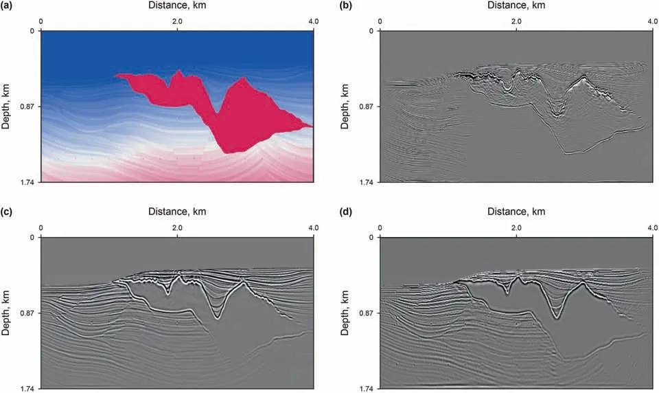
Fig.6.The SigsBee2A model (a) and the imaging results from GBM (b),RTM (c) and LSRTM (d).

Fig.7.Magnified views in Fig.6a (a),6b (b),6c (c) and 6d (d).

4.Future perspective

At present,the main challenge of seismic imaging is to produce high-precision images for low-quality data,extremely deep reservoirs,and dual-complex structures(LED subsurface imaging).In the future,it will have broad development prospects in the following aspects.

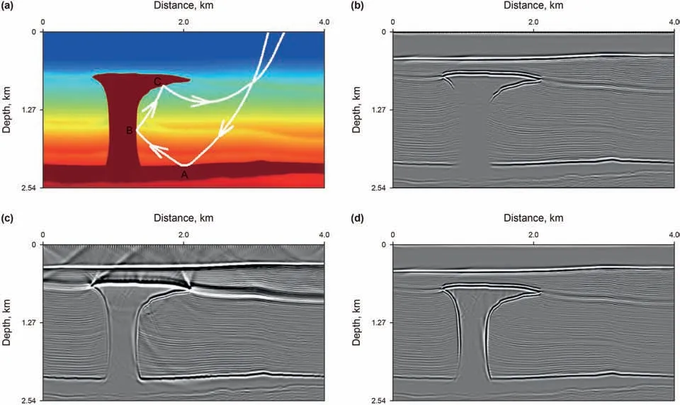
Fig.8.The BP model (a) and the imaging results from GB (b),RTM (c) and LSRTM (d).

Fig.9.Migration velocity model (a) and imaging results from GBM (b) and RTM (c) and LSRTM (d).

4.1.Research progress on the attenuation-compensated imaging method

The Earth has strong viscosity.Ignoring viscosity results in weak amplitude and misplacement of reflectors in images (Aki and Richards,2002;Carcione,2007),the attenuation compensation mainly includes the following two categories:

4.1.1.Inverse Qfiltering technology

Inverse Q filtering technologies are implemented based on the wavefield continuation (Zhang et al.2007a,2013),the series expansion (Bickel and Natarajan 1985;Pei and He,1994;Gao and Ling,1996),the phase correction (Hargreaves and Calvert,1991;Bano,1996) and both the phase correction and amplitude compensation (Futterman,1962;Hale,1981;Varela et al.,1993).Although these inverse Q filtering methods are effective and have high computational efficiency,they cannot accurately compensate for attenuation in complex geological structures.

4.1.2.Q migration technology

With the development of migration technology,the inverse Q migration technology has become a research hotspot.

Inverse Q migration has been implemented with the ray-based method (Traynin and Reilly,2008;Xie et al.,2009),one-way wave equation method (Dai and West,1994;Zhang and Wapenaar,2002;Zhang et al.,2013;Sun and Fu,2013;Guo and Lou,2014),RTM method (Deng and McMechan,2007;Bai et al.,2013;Zhu et al.,2014;Zhou et al.,2018;Qu and Li,2019) and LSRTM method(Li et al.,2014;Dutta and Schuster,2014;Dai et al.,2015;Sun et al.,2016;Chen et al.,2017;Yang and Zhu,2019;Qu et al.,2021).For the Q-compensated RTM,when compensating the wavefield decay in the attenuating medium,high-frequency noise will grow exponentially with time,resulting in instability(Zhang et al.,2010;Fletcher et al.,2012;Bai et al.,2013;Zhu et al.,2014).To solve this problem,the regularization operator method(Zhang et al.,2010),the high-pass filtering method(Zhu et al.,2014)and the adjoint operator method(Dutta and Schuster,2014;Li et al.,2014)are proposed for stabling backward-propagation.Figs.10 and 11 show a numerical example of Q-compensated LSRTM with viscoacoustic data for a salt model (Li et al.,2014).

4.2.Research progress on imaging in the anisotropic medium

Alkhalifah(1998)made an acoustic approximation of the elastic wave equation and deduced the fourth-order pseudo-acoustic wave equation in vertical transverse isotropy(VTI)media according to the dispersion relation approximation theory.Zhou et al.(2006)simplified the fourth-order qP wave equation in VTI media to a second-order form by introducing various forms of auxiliary wavefields.To improve the accuracy of calculating wavefield in VTI media,Hestholm (2009) further proposed the first-order qP wave equation of VTI media.Recently,some anisotropic quasi-acoustic LSRTM methods are proposed based on the adjoint state theory(e.g.Li et al.,2017d;Zhu et al.,2018;Huang and Li,2019;Guo et al.,2019;Mu et al.,2020).Qu et al.(2017a) proposed a viscoacoustic anisotropy LSRTM.Figs.12 and 13 show a numerical example of prestack pure-qP wave RTM of the 2D BP2007 TTI model (Huang and Li,2017).

4.3.Research progress on imaging for surface topography

Fig.10.A salt model.(a) Velocity model;(b) Q model;(c) Background velocity model;(d) Slowness perturbation (Li et al.,2014).

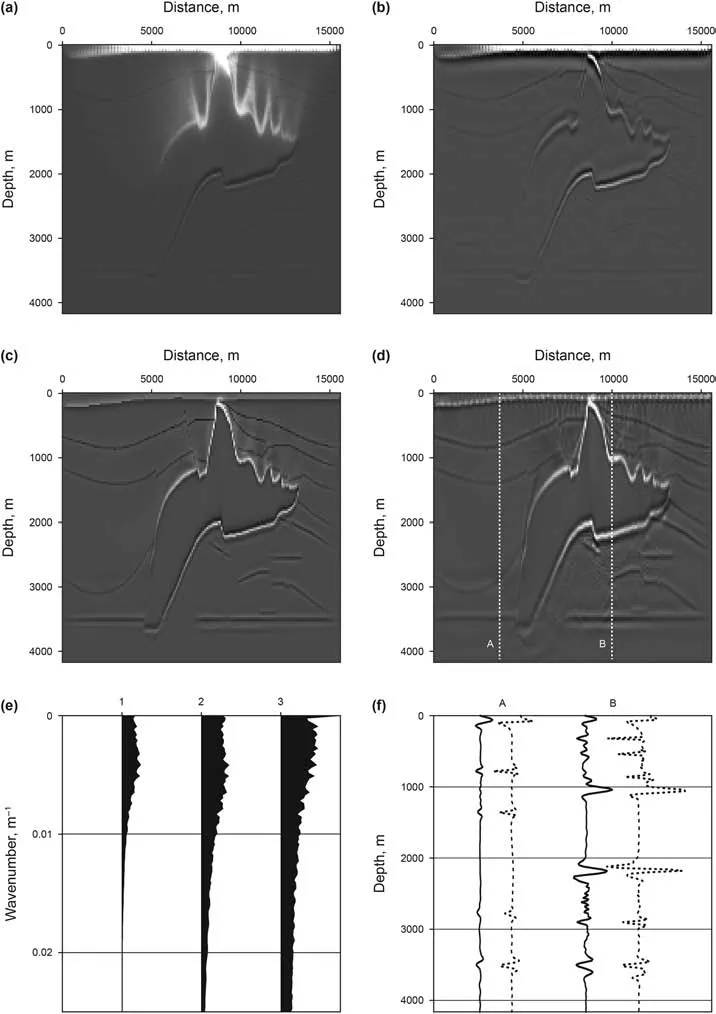
Fig.11.Comparison of image results of salt model.(a) Image result at 1st iteration;(b) applying high-pass filtering to Fig.11a;(c) Image result at 50th iteration of viscoacoustic LSRTM;(d)Image result at 50th iteration of acoustic LSRTM;(e)Comparison of wavenumber spectrums,where the trace numbered with 1,2,3 is the wavenumber spectrum of the image result of acoustic LSRTM,viscoacoustic LSRTM,ideal image result,respectively;(f)Comparison of image result in Fig.11c(dash line)and 11d(real line)at location A and B(Li et al.,2014).

Extreme surface topography brings a great challenge to imaging subsurface structures.The commonly used elevation static correction method based on the assumption of surface consistency is not applicable.The ray imaging methods have good adaptability to complex near-surface conditions and can directly carry out wavefield continuation and migration imaging on the undulating surface(Wiggins,1984;Gray,2005;Jager et al.,2003;Yue et al.,2012;Yang et al.,2015a,2015b;Huang et al.,2015a,2015b).For wave-equationbased RTM and LSRTM methods,wavefield continuation operators based on the finite-difference method (FDM) (Li et al.,2019),the finite-element method (FEM) (Moczo et al.,1997),the pseudospectral method (PSM) (Fornberg and Ghrist,1999),the spectralelement method (SEM) (Madec et al.,2009) and the grid method(GM)(Zhang,2004)have been constructed to produce topographic wavefields.Among these methods,FDMs have been widely introduced to implement LSRTM because of their robustness,high computational efficiency,small memory storage and easy implementation.RTM and LSRTM based on the conventional finitedifference operator use uniform rectangular grids to simulate forward-propagated source wavefields and backward-propagated receiver-side wavefields,leading to strong scattering and diffracted noise.Therefore,some curvilinear grid schemes(Hestholm and Ruud,1994;Zhang and Chen,2006;Qu et al.,2017b),variable grid scheme (Jastram and Behle,1992;Huang et al.,2015a,2015b)and various coordinate systems(Shragge,2009;Ma and Alkhalifah,2013;Zhu et al.,2019) are developed to improve the accuracy and efficiency of seismic wavefield continuation.Fig.14 shows a numerical example of topographic QRTM on a modified attenuating Marmousi model with irregular surface (Qu and Li,2019).

Fig.12.2D TTI BP2007 model of velocity v (a),dip parameter θ (b),Thomsen parameter ε (c) and δ (d).

Fig.13.Prestack pure-qP wave RTM image of the 2D BP2007 TTI model(Huang and Li,2017).

4.4.Research progress on elastic multi-component imaging

Multi-component seismic data contain more target structure information (Jin et al.,1998;Xie and Wu,2005) and maintain the kinematics (travel time,path,etc.) and dynamics (waveform,amplitude,frequency,phase and polarization characteristics,etc.)properties of the seismic wavefield (Ma et al.,2011).Due to the existence of shear waves,multi-component seismic data can better identify the reservoir fluid,estimate the fracture distribution,and analyze the anisotropy (Du et al.,2012).

Therefore,multi-component seismic data migration imaging is an effective technique for imaging complex subsurface structures(O'Brien and Gray,1996;Rosenberg,2000;Glogovsky et al.,2002;Ravasi and Curtis,2013;Wang et al.,2013).For elastic wave migration,RTM is still a common choice(Baysal et al.,1983;Levin,1984;Chang and McMechan,1986,1987,1994;Zhe and Greenhalgh,1997;Yoon and Marfurt,2006;Sun and McMechan,2001,Sun et al.,2006;Du and Qin,2009;Yan and Xie,2012).

Sun and McMechan (2001) proposed to use the acoustic RTM process to deal with the elastic wave data.Firstly,the elastic wave seismic data is separated into P-and S-waves,and then the acoustic RTM is carried out separately for the two wave modes.Sun et al.(2006)extended this approach to a 3D case.Elastic RTM(ERTM)is a better choice to migrate for multi-component data (Sun and McMechan,1986;Chang and McMechan,1994;Zhe and Greenhalgh,1997;Yan and Sava,2008;Qu et al.,2015),implemented by the forms of scalar (e.g.Sun and McMechan,2001,Sun et al.,2006) and vector ERTM (e.g.Gu et al.,2015).Among these,the vector ERTM method can correctly deal with the transformation between wave modes,and completely maintain the vector characteristics of seismic waves in the wavefield reconstruction.Therefore,vector imaging is the development trend of ERTM.However,crosstalk noise between P-andS-wavewill cause severeartifacts in multicomponent images (Yan and Sava,2008).To reduce the imaging crosstalk artifacts,P-and S-wave modes should be separated in the forward-and backward-wavefield (Yan and Sava,2008).In an isotropic medium,P-and S-wavefield can be easily separated by using the Helmholtz decomposition to calculate divergence and curl fields to the full wavefields (Aki and Richards,2002),however changing the amplitude and phase attributes(Sun and McMechan,2001;Sun et al.,2006).Besides,in this method,polarity reversals should be corrected in PS and SP images(Balch and Erdemir,1994;Du et al.,2012).Vector ERTMs based on the decoupled P-and S-wave equations are proposed (e.g.Gu et al.,2015;Du et al.,2017) to overcome these above problems.Thus,Elastic LSRTM(ELSRTM)has been rapidly developed in recent years(e.g.Chen and Sacchi,2017;Duan et al.,2017;Feng andSchuster.2017;Ren et al.,2017;Rochaand Sava,2018;Sun et al.,2018;Feng and Huang,2020).To suppress the crosstalk noise between P-and S-wave in ELSRTM,various ELSRTM methods based on the wavefield separation have been gradually developed(Gao et al.,2017;Gu et al.,2018;Qu et al.2018,2019b;Guo and McMechan,2018;Yang et al.,2019;Konuk and Shragge,2020).Figs.15-16 illustrate a numerical example of ERTM and ELSRTM on Marmousi2 model(Gu et al.,2018).

4.5.Research progress on geological target-oriented imaging

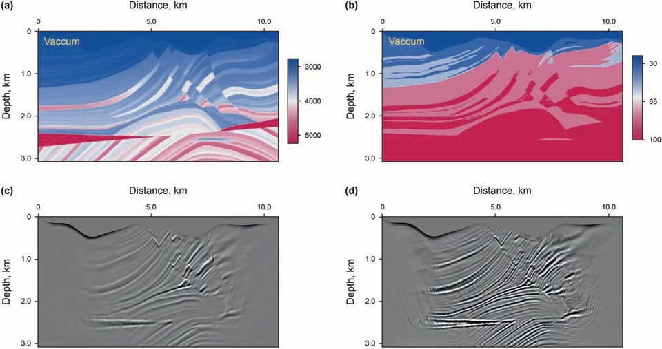
Fig.14.Topograhic attenuating Marmousi velocity (a) and Q (b) models,and images obtained from noncompensated (c) and Q-compensated (d) RTM (Qu and Li,2019).

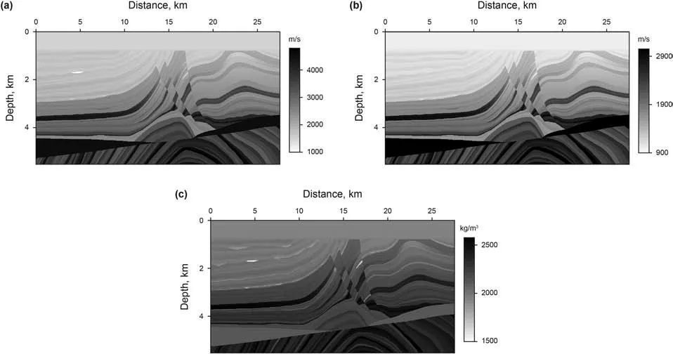
Fig.15.Marmousi2 model of P-velocity (a),S-velocity (b) and density (c).

In recent years,the computational cost of seismic imaging became more and more expensive due the continuous increase of complexity of imaging algorithms.Geophysicists begin to focus imaging on local targets.In general,geological target-oriented imaging methods can be divided into model-selective local target imaging methods (e.g.Tang and Biondi,2011;Maranganti and Agnihotri,2014) and data-selective local target imaging methods(e.g.Araya et al.,2016).

4.5.1.The model-selective local target imaging method

Model-selective local target imaging methods are mainly as follows:(1)the special observation system method.The main idea of this method is to place the observation system closer to the target.(2) Data datum reconstruction method.It reconstructs conventional seismic data to the vicinity of the target (Berryhill,1984;Bakulin and Calvert,2006;Dong et al.,2009;Wapenaar et al.,2014;Ravasi et al.,2016;Guo and Alkhalifah,2020).The imaging quality of the target depends on the accuracy of the Green function estimation between the surface and the target area.(3)Acoustic-elastic coupled wavefield continuation method.This method uses elastic waves in some areas and acoustic waves in other areas(Willemsen and Malcolm,2017).This method is usually applied in the simulation and imaging of ocean bottom seismic(OBS)data in deep-sea environments(e.g.Choi et al.,2008;Madec et al.,2009;Qu et al.,2017b,2020a).(4) Seismic imaging optimization algorithm guided by geological target.This method improves the original operator by proposing a geological target-oriented operator to increase the imaging efficiency (Valenciano et al.,2006;Tang,2009;Malcolm and Willemsen,2016;Wang et al.,2017).

Fig.16.Imaging results in PP-(a) and PS-(b) component from ERTM and in λ-(c) and μ-(d) component from ELSRTM (Gu et al.,2018).

4.5.2.The data-selective local target imaging method

Data-selective local target imaging methods include prismatic wave,multiples,diffraction wave imaging,etc.

(1) Prismatic waves imaging

Prismatic waves may illuminate steeply dipping structural areas where primaries cannot be acquired.Therefore,prismatic waves can be used to improve the illumination and imaging effect on steeply dipping structures (Farmer et al.,2006;Malcolm and De Hoop,2010,Malcolm et al.,2011;Qu et al.,2016).Although the energy of prismatic waves is much weaker than that of primaries,by using prismatic waves,RTMs still can construct subsurface images with higher precision and resolution in steeply dipping structural regions poorly illuminated by primaries (Dai,2012;Liu and Weglein,2014;Deeks and Lumley,2015).

(2) Imaging of multiples

Multiples have a longer travel path and a smaller reflection angle than primaries,so they have a wider transverse illumination area and a higher vertical resolution.Multiples imaging can be broadly classified into four categories.Firstly,the multiples are converted into quasi-primaries and then migrated.This multiples imaging method is implemented with ray migration (Reiter et al.,1991;He et al.,2007) or wave equation migration (Berkhout and Verschuur,2003;Verschuur and Berkhout,2005).Secondly,loworder multiples are used as seismic sources to achieve high-order multiples imaging (e.g.Youn and Zhou,2001;Liu et al.,2011b).Figs.17 and 18 show an example of imaging of different-order multiples (Li et al.,2017e).Thirdly,Marchenko imaging (e.g.Slob et al.,2014;Wapenaar et al.,2017;Lomas et al.,2020).Fourthly,least-squares multiples imaging.It mainly includes the ray-based least-squares migration of multiples (Brown and Guitton,2005)and LSRTM of multiples(Wong et al.,2015;Tu and Herrmann,2015;Liu and Liu,2016;Qu et al.,2020b,2020c;Li et al.,2020b).

(3) Diffraction wave imaging

There are two types of diffraction imaging methods:direct and indirect imaging by using diffractions.The direct imaging methods mainly include the Kirchhoff methods(Kozlov et al.,2004;Wu et al.,2007a;Moser and Howard,2010;Koren and Ravve,2010;Sun et al.,2014),the angle-domain methods (Zhu and Wu,2010;Bai et al.,2011;Reshef,2008;Reshef and Landa,2009).In this method,the energy of the diffraction is directly separated in the imaging process according to the energy difference between the reflections and the diffractions.The indirect methods produce theimagingof diffraction step-by-step:firstly,the diffractions should be separated from prestack gathers,such as,common-shot,plane-wave,common-offset gathers,etc.Then,diffraction waves will be imaged individually.The indirect diffraction imaging method mainly includes commonoffset gather methods(Landa et al.,1987),common diffraction point profile methods(Kanasewich and Phadke,1988),common-shot record methods (Nowak,2005;Khaidukov et al.,2004;Moser and Howard,2010),plane wave record methods (Taner et al.,2006)and others(Papziner and Nick,1998;Bansal and Imhof,2005).

5.Conclusions

Fig.17.Velocity model(a)and separation results of different-order multiples for the complex model.(b)Single shot record,(c)the separated primaries,(d)the separated first-order multiples,(e) the separated second-order multiples,and (f) the separated third-order multiples (Li et al.,2017e).

Fig.18.Imaging results from RTM with (a) and without (b) multiples (Li et al.,2017e).

Imaging technology has always been a hot but difficult topic,as well as,set in the central stage in the field of seismic exploration.In recent years,with the progress of oil and gas exploration,exploration targets have also become more and more complex.It challenges our imaging technologies immensely and forces the development of seismic imaging technologies to adapt to the complex irregular surface,intense variation of velocity,poor illumination in subsalt areas,and small-scale and steeply dipping structures,etc.Compared with the stacking-and migration-based imaging methods,the inversion-based imaging methods produce a better image with higher spatial resolution,fewer migration artifacts,and better-balanced reflector amplitudes.Although the inversion-based imaging methods show huge promise to improve the imaging quality significantly,they still need to improve computational efficiency,reduce the dependence on the migration velocity and wavelets,and mitigate the sensitivity to noise.In the future,the seismic imaging technology will have broad development prospects,including attenuation-compensated imaging,anisotropic imaging,imaging with surface topography,elastic multi-component imaging,and geological target-oriented imaging.

Acknowledgment

This research is supported by seismic wave propagation and imaging (SWPI) group of China University of Petroleum (East China).This research is supported by National Natural Science Foundation of China (42174138,41904101,42074133),Natural Science Foundation of Shandong Province (ZR2019QD004),Fundamental Research Funds for the Central Universities (19CX02010A),the Major Scientific and Technological Projects of CNPC (ZD 2019-183-003) and Talent introduction fund of China University of Petroleum(East China) (20180041).