Machine learning and numerical investigation on drag reduction of underwater serial multi-projectiles

Xi Huang, Cheng Cheng, Xiao-bing Zhang

School of Energy and Power Engineering, Nanjing University of Science and Technology, Nanjing, 210094, China

Keywords:Drag reduction Serial multi-projectiles Machine learning Artificial neural network (ANN)Numerical simulation

ABSTRACTTo increase launching frequency and decrease drag force of underwater projectiles, a serial multiprojectiles structure based on the principle of supercavitation is proposed in this paper.The drag reduction and supercavitation characteristics of the underwater serial multi-projectiles are studied with computational fluid dynamics (CFD) and machine learning.Firstly, the numerical simulation model for the underwater supercavitating projectile is established and verified by experimental data.Then the evolution of the supercavitation for the serial multi-projectiles is described.In addition, the effects of different cavitation numbers and different distances between projectiles are investigated to demonstrate the supercavitation and drag reduction performance.Finally,the artificial neural network(ANN)model is established to predict the evolution of drag coefficient based on the data obtained by CFD,and the results predicted by ANN are in good agreement with the data obtained by CFD.The finding provides a useful guidance for the research of drag reduction characteristics of underwater serial projectiles.

1.Introduction

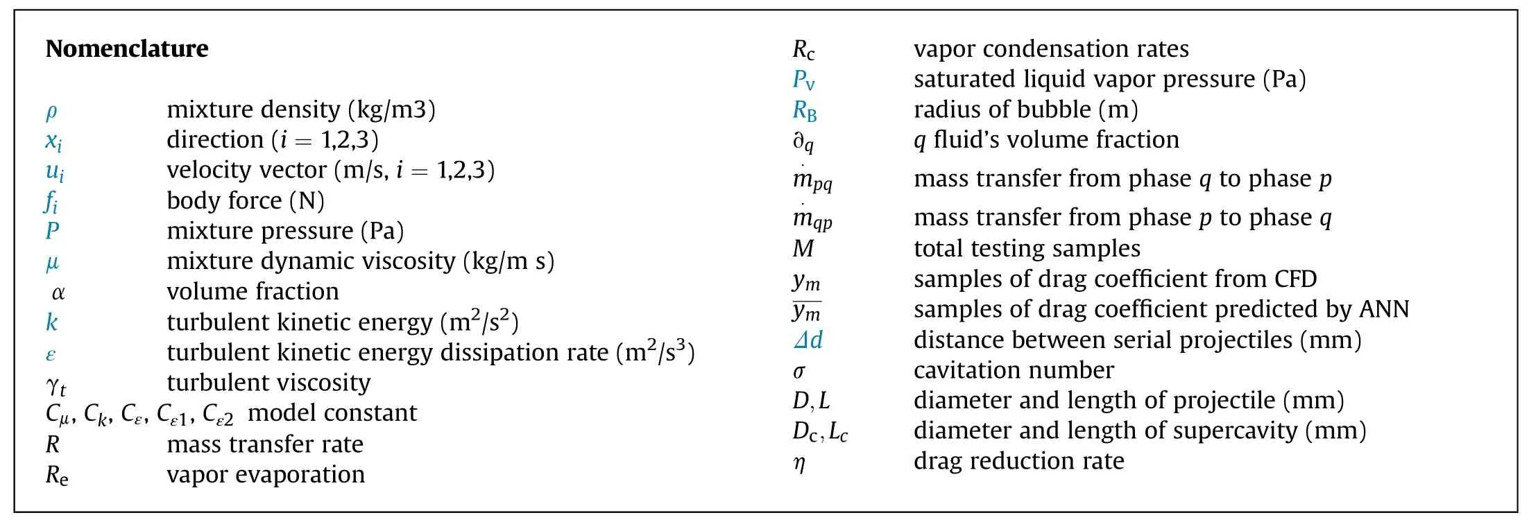
The quest to achieve high launching frequency and higher speed is one of the key goals for researchers in the field of underwater projectiles.Many methods have been proposed for reducing the drag force to reach higher speed,such as using a superhydrophobic surface[1],using a compliant surface[2,3],and so on[4,5].One of the most effective methods is supercavitating drag reduction technology,which can be used to achieve a significant reduction of hydrodynamic drag by wrapping a large,continuous cavity around the underwater projectile[6,7].The supercavitating drag reduction technology shows great performance to defense against frogloks,torpedoes, mines, etc.

The supercavitating drag reduction technology has been widely investigated.For instance,Ceccio[8]reviewed the use of partial and supercavity for drag reduction of axisymmetric objects moving within liquid.Cavitator with different shapes have been used to investigate the drag reduction effects for the supercavitating flow[9-11].Several studies of supercavitation influenced by turbulent drag-reducing additives have been widely discussed by researchers[12-14].In general, these studies are focused on single vehicle in supercavitating flow.

Researches on multi-projectiles in air have been investigated to improve the launch frequency [15-18].Recently, the supercavitating flow for underwater multi-projectiles have been reported.The supercavitating flow field of continuously fired projectiles was studied by Shi [19].The evolution of cavity shape and the interaction between two cylinders in series and parallel was investigated in Ref.[20].The influences of serial distance on the bubble shape, flow field characteristics and projectile motion law were explored in Ref.[21].These researches effectively prove that the drag force can be reduced with underwater multiple vehicles.However, the matching relationships of serial multi-projectiles between different conditions (cavitation number, distance between projectiles, etc.) and the drag characteristics have not been investigated, because obtaining the relationship between drag characteristics and different conditions requires simulation time and extensive calculations.

?

Machine learning has an obvious advantage in computational efficiency, which also has been applied in the field of fluid mechanics.An algorithm for learning velocity and pressure fields from flow visualization was proposed by Maziar [22].The model averaging neural networks (MANN) were set up to find the relationships between the unknown closure terms and the resolved average variables in Ref.[23].The depth neural network model was used to calculate the Reynold average turbulence model and the anisotropic component of Reynolds stress by Ling [24].A datadriven, physics-informed machine learning approach for reconstructing discrepancies in RANS modeled Reynolds stresses was proposed in Ref.[25].

In this paper, a serial multi-projectiles structure for drag reduction is proposed and machine learning is applied to investigate the drag characteristics of serial multi-projectiles.In the numerical simulation,the natural supercavitation phenomenon of the serial projectiles is investigated.This study also focuses on investigating the effects of different cavitation numbers and different distances between serial projectiles.Finally, the artificial neural network (ANN) model is established to predict the evolution of drag coefficient based on the data obtained from CFD.

2.Drag reduction principle of serial multi-projectiles structure

A new serial multi-projectiles structure (see Fig.1) for drag reduction is proposed in this section.The structure can be applied in the field of underwater launching to realize high launching frequency and reduce the drag of underwater projectiles to improve the performance.The structure includes: barrel, main body, projectile, holder, vent, chamber, cavity and piston.The launching processes are as follows:

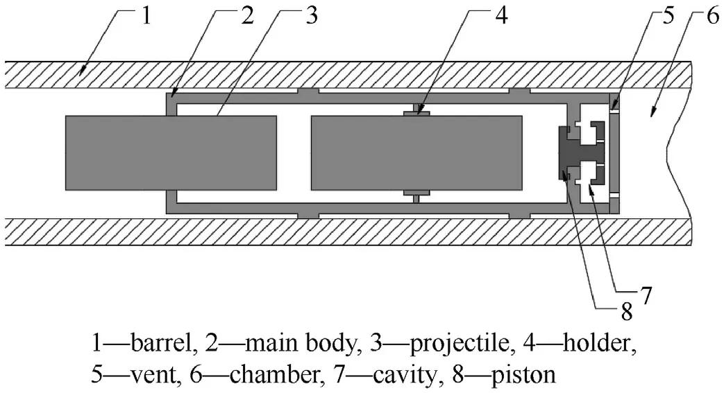
Fig.1.A serial multi-projectiles structure for drag reduction.

(a) At the beginning, the propellant in the chamber is ignited and produces high temperature and high-pressure gases,which pushes the main body forward in the gun barrel.Then,high temperature and high-pressure gases flow into the cavity through the vent.The pressure in the cavity increases and the piston moves.

(b) After the piston moving, the high temperature and high pressure gases flow into the main body through the hole on the piston.When the main body leaves the muzzle,the main body disintegrates and the two projectiles separate from the main body due to the pressure difference between the inside and outside of the main body.

(c) When the two projectiles enter water, the flow field around the two projectiles will interact with each other and the supercavitation will be generated.Then the drag force of the projectiles will be reduced based on the supercavitating drag reduction technology.

3.Mathematical methods

3.1.CFD mathematical methods

(a) Governing equations

To obtain the velocity and pressure fields,the equations of mass and momentum conservation were solved.The governing equations of continuity equation and momentum equations for the mixture can be written as:

where, ρ is the mixture density,is time. x（=1，2，3） is the direction, and uis the velocity vector.fis the body force,is the mixture pressure, and μ is the mixture dynamic viscosity.α is the volume fraction, and subscripts v and l indicate ‘‘vapor’’ and‘‘liquid,’’respectively.μis vapor dynamic viscosity and μis liquid dynamic viscosity.ρis vapor density and ρis liquid density.

(b) Turbulent model

turbulent kinetic energy dissipation rate ε is as follows:

where,the model constants,C,,andare 0.09,0.1,0.08,144 and 1.92, respectively.

(c) Cavitation model

The Schnerr-Sauer cavitation mode was proposed by Schnerr and Sauer [27], and they used a similar method to derive the expression of liquid water changing into vapor accurately.The equation for the vapor volume fraction can be expressed as follows:

where,is mass transfer rate.is the vapor evaporation andis the vapor condensation rates.is the saturated liquid vapor pressure,is the radius of bubble and= 1× 10.

(d) Volume of Fluid (VOF)model

The VOF model [28]can solve a single set of momentum equations and track the volume fraction of each fluids throughout the domain to model two or more immiscible fluids.For each phase added,only the volume fraction of the term changes.In short,if thefluid’s volume fraction in the cell can be expressed as ∂,then the following three conditions are:

(1) ∂= 0, the cell is empty;

(2) ∂= 1, the cell is full;

(3) 0<∂<1, the cell is a mixing domain offluid and one or more other fluids.VOF model can capture the interface of different fluids by solving the continuous equation of volume fraction of one or more fluid phases.The equation is as follows：

3.2.ANN mathematical methods

Fig.2 shows the multi-layer feed-forward neural network in this paper.In the feedforward neural network,the neurons in each layer can receive the signals from the neurons of the previous layer and output the signals to the next layer.The network consists of three layers: input layer, hidden layer and output layer.The 0 layer (the input layer) contains the input eigenvector; the last layer (the output layer) contains the output vector; another intermediate layer is the hidden layer, and the number of hidden layers can be one or more.There is no feedback in the whole network, and the signal propagates from the input layer to the output layer in one direction[29].

Network performance is evaluated by mean squared error(MSE)of the training data.It is used to test the deviation between the real value and the predicted value of the model,and it is shown by the following equation:

4.Numerical methods and validations

4.1.Numerical methods

The computational fluid dynamics software ANSYS FLUENT 17.0[28]is used to perform the numerical simulation of supercavitating flow.The numerical simulation uses a pressure-implicit solver.The pressure-velocity coupling algorithm is set to be SIMPLE scheme.In addition, the standard-ε model is adopted as turbulent model,and VOF multiphase flow model is used as the computational model.In the numerical simulation, the Schnerr-Sauer cavitation model is selected as the mass transport model between liquid water and steam.

Fig.2.A multi-layer feed-forward neural network.

Machine learning is often based on a large number of data,otherwise the network model will be over fitting.For machine learning,the more data,the more likely to improve the accuracy of the model.In this paper,to train the machine learning drag model,drag force data from CFD is collected around the second projectile underwater serial projectiles.The drag coefficient data obtained from CFD is randomly divided into three kinds of samples:training samples(70%),validation samples(15%)and testing samples(15%).The training samples are presented during training, and the network is adjusted according to its error.The validation samples are used to measure network generalization, and stop training when generalization fails to improve.Rest of the testing samples are not used during training but are used to further check the performance of the network.In this paper, all the ANN setup,training and prediction are carried out in the MATLAB neural network toolbox.Table 1 shows the ANN settings, inputs and results.Where,is moment, σ is cavitation number, Δis distance between serial projectiles andis the drag coefficient of the second projectile of the serial projectiles, respectively.

Table 1ANN simulation settings, inputs and results.

Table 2Grid convergence results.

4.2.Computational domain and boundary conditions

In the numerical simulation, the model is simplified as an axisymmetric two-dimensional model.The computational region and boundary conditions are shown in Fig.3.The diameter() of projectile is 6 mm and the length () of projectile is 30 mm.The length of computational region is 500 mm and the width is 200 mm.The mesh of the computational domain is the structured grid.The distance between two projectiles is defined as Δ.Additionally,a velocity inlet condition is imposed on the inlet boundary,and a pressure outlet condition is imposed on the outlet boundary.The no-slip wall boundary condition is imposed on the projectile surface and the upper boundary.

4.3.Experimental verification

An experiment verification case of underwater high-speed projectile is used to verify the accuracy of numerical methods.The free-stream velocity is 970 m/s and the free-stream pressure is 1.4×10Pa.The length()of the high-speed projectile is 157.4 mm with a disk cavitator radius of 0.71 mm and base radius of 6.56 mm.Fig.4 presents comparisons of cavity shape between numerical simulation and experiment of Hrubes [30].The comparisons of cavity thickness between experiment and numerical simulation are shown in Fig.5.The calculated results by CFD show a good agreement with the experimental data.The simulation results can be reliable by the proposed approach.

4.4.Grid independence

Fig.3.Computational region and boundary conditions

Fig.4.Comparisons of cavity shape between numerical simulation and experiment.

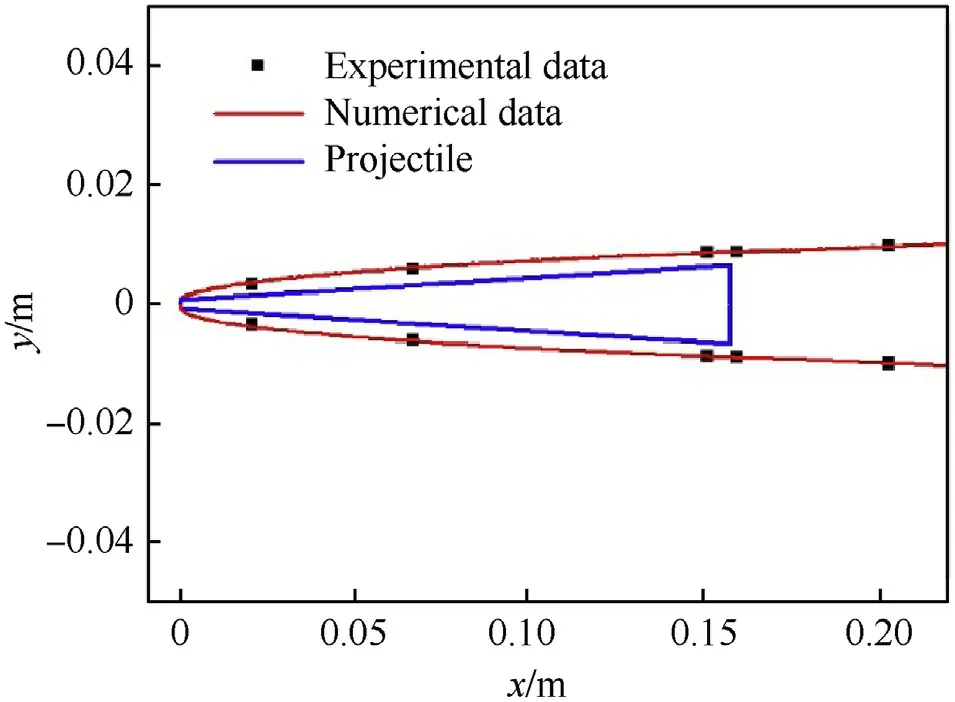
Fig.5.Comparison of cavity thickness between experiment and numerical simulation.

The grid convergence studies are investigated to discuss the effect of the gird size.The grid size varies to be 10,648, 33,780,66,616,135,210,247,062 and 313,676.Grid convergence results are given in Table 2.The relative error decreases with the grid size.When the grid size is 247,062, the relative error is only 0.33%.Although further increasing the grid size can reduce the error a bit,the computational time increases significantly.By balancing the computational time and numerical accuracy,the gird size 247,062 is sufficient to ensure the numerical accuracy and the grid independent results.

5.Results and discussions

5.1.Numerical simulation results

(a) Evolution of cavitation

The evolution of cavity configurations with the distance of 4 L and σ of 0.0215 is shown in Fig.6.It can be seen that at=0.2 ms,the cavitation occurs around the head and tail of the serial projectiles,resulting in cavitation inception in this region.The lengths of the cavity around the head and the tail of the projectiles increase with the time.As a result, the cavity around the head and the tail gradually merge.At the instant of 0.6 ms，the first and the second projectile form supercavity independently.After that,at the instant of 5 ms, the first and the second supercavity are fused.And at= 11 ms, the supercavity completely wraps around the serial projectiles.

Fig.7 shows the pressure contours of serial projectiles at= 3 ms and= 7 ms, respectively.As is shown in Fig.7(a), the maximum pressure value of the projectile surface appears at the head of the projectile and the pressure of projectile body and tail is small, resulting in low pressure area.At the instant of 3 ms, drag force before the second projectile is smaller than that of first projectile, and the point of vapor collapse is farther to the second projectile.Thus, the size of the second projectile supercavity is larger.At the instant of 11 ms, the second projectile is completely wrapped by the supercavity generated by the first projectile,which can be found in Fig.6(c) and (f).

Fig.8 shows the drag coefficient with a distance of 4L and σ of 0.0215.The drag coefficients decrease sharply at first,which is due to the supercavity generated around two projectiles.The drag coefficients keep stable when supercavity fused.It can be seen that the drag coefficient of the second projectile is smaller than that of the first projectile,indicating that the structure of serial projectiles reduces the drag force of the second projectile.

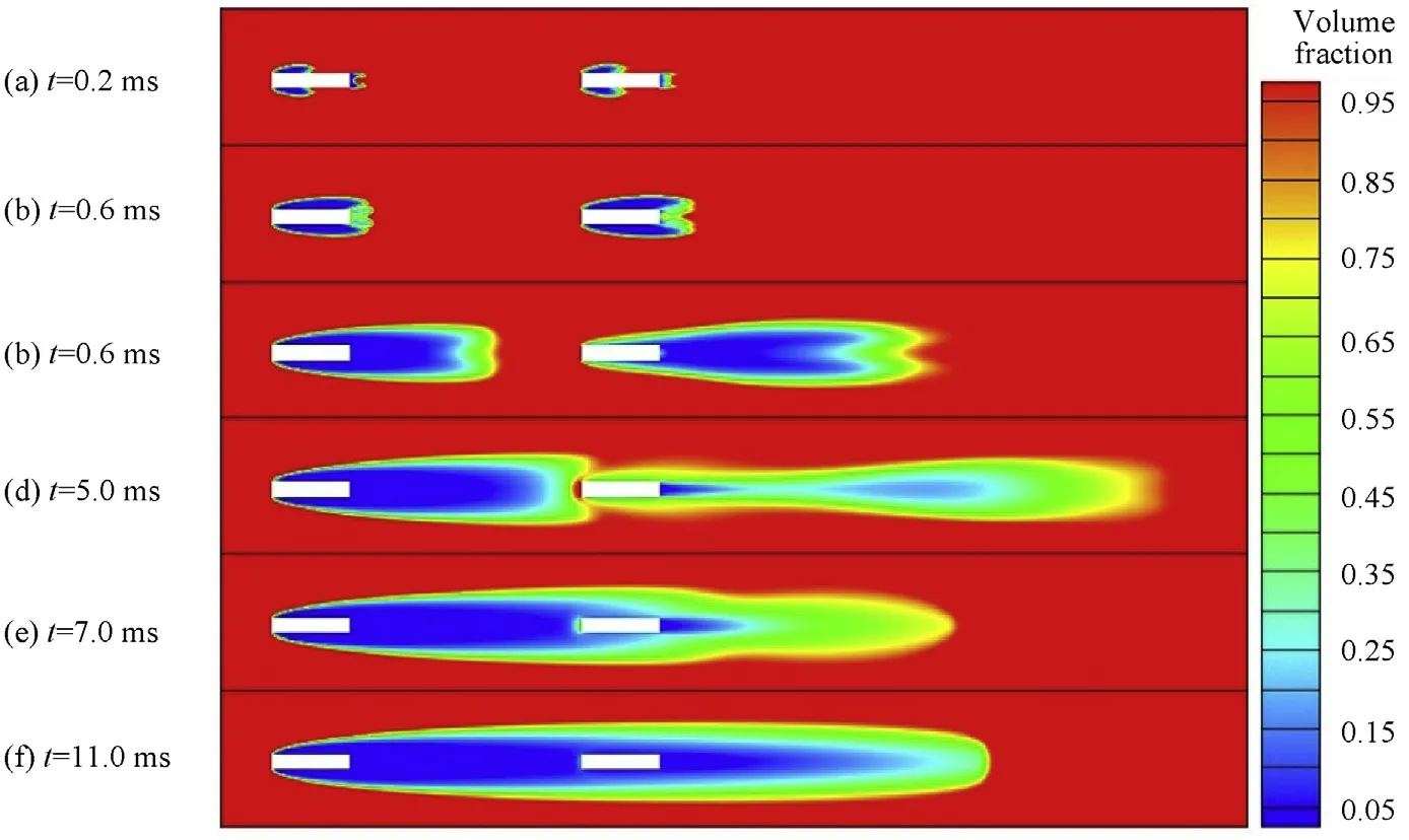
Fig.6.Evolution of cavity configuration.

Fig.7.Pressure contours of serial projectile.

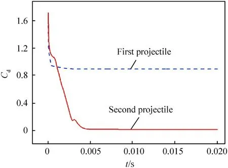
Fig.8.Drag coefficient at a distance of 4L and σ of 0.0215.

Fig.9.Outlines of supercavity under different cavitation numbers.

(b) Effects of different cavitation numbers

Fig.9 shows the outlines of supercavity under cavitation number of 0.0215,0.0266,0.0336 and 0.0439,respectively.As is shown in Fig.9, the length and diameter of supercavity increase with the decreasing of the cavitation number.When the cavitation number is 0.0439, the first and second projectiles form complete supercavity respectively.The length and aspect ratio of supercavity with different cavitation numbers are shown in Fig.10.The length and aspect ratio of supercavity decrease with the increasing of the cavitation number.

To analyze the drag reduction characteristics of serial projectiles,Fig.11 shows the drag coefficient and drag reduction rate of serial projectiles under different cavitation numbers.It can be seen that with the increasing of cavitation numbers,the drag coefficient of the second projectile increases and the drag reduction rate decreases.When the cavitation number is greater than 0.0336, the supercavity of the first projectile cannot completely wrap the second projectile, and the second projectile forms independent supercavity, so that the drag coefficient of the second projectile increases sharply.The drag reduction rate η is expressed by the following formula:

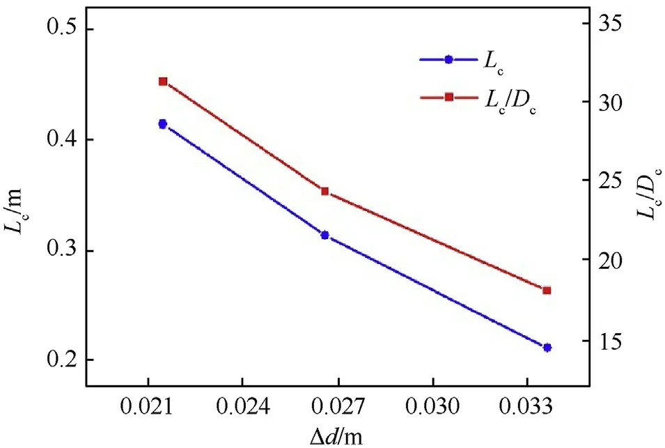
Fig.10.Supercavity length and aspect ratio under different cavitation numbers.

Fig.11.Drag coefficient and drag reduction rate of serial projectiles under different cavitation numbers.

where,is the drag coefficient of a single projectile under the same working conditions, andis the drag coefficient of the second projectile of the serial projectiles.

(c) Effects of different distance

The length and aspect ratio of supercavity under different distances (Δ= 120 mm,180 mm, 240 mm, 300 mm, 360 mm) are shown in Fig.12.It can be concluded that the trend of supercavity length is consistent with the aspect ratio.The length and aspect ratio of supercavity increase with the increasing of the distance between serial projectiles.Fig.13 shows the drag coefficient and drag reduction rate of serial projectiles under different distances.With the increasing of distances,the drag coefficient of the second projectile increases and the drag reduction rate decreases.When the distance is greater than 8L,the supercavity of the first projectile cannot completely wrap the second projectile due to the long distance.And the second projectile forms independent supercavity,so that the drag coefficient of the second projectile increases sharply.

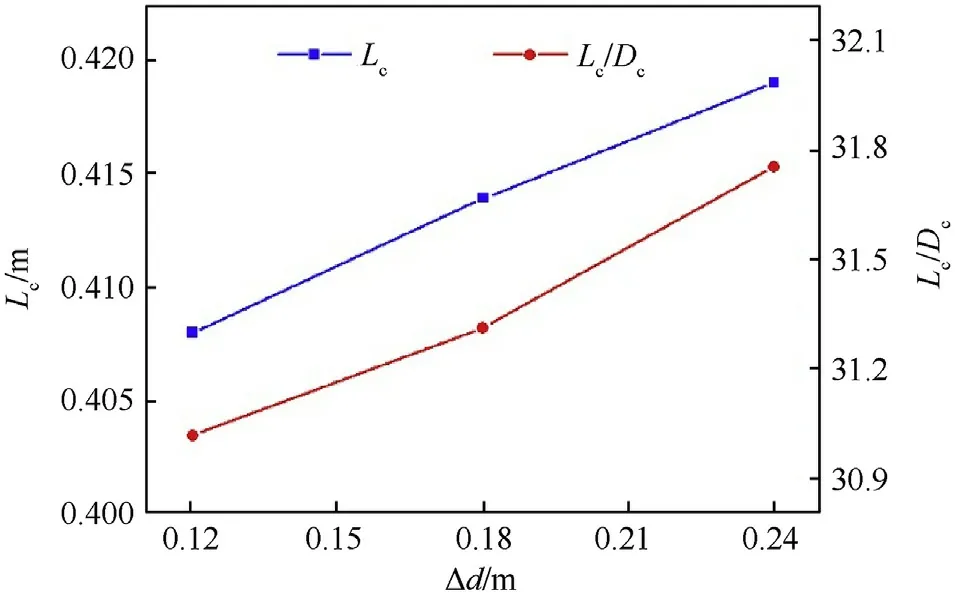
Fig.12.Supercavity length and aspect ratio under different distances.

5.2.ANN prediction results

The neural network model is calculated based on the results of 39,992 data computed by CFD, including 27,994 data randomly selected as training samples, 5999 data selected as validation samples and 5999 data selected as testing samples.Table 3 shows the mean square error of the samples.The mean square errors of the training,validation and testing samples are around the order of 10,indicating that the model can work with high accuracy.There is no significant difference between the training samples,validation samples and testing samples, which means that the trained ANN model is not over fitted by the training data or validation data.

Table 3Mean square errors of the samples.

The ANN predictions for the training samples, validation samples, testing samples and all samples are shown in Fig.14.The xaxis represents the data computed by CFD, and the-axis represents the prediction results of ANN.The regressionvalues of training, validation and testing samples are all above 0.99, which shows that the current model can estimate the drag coefficient of the whole range.

Fig.15 shows the error histogram of training samples,validation samples, testing samples.It can be seen that most of the training errors are near zero, and the number of training errors decreases rapidly with the increasing of the error.The distribution is almost normal, the peak is in the middle, and the left and right sides are roughly symmetrical.The error histogram suggesting the ANN model has a high accuracy in prediction.

Fig.13.Drag coefficient and reduction rate of serial projectiles under different distances.

Fig.16 shows the comparisons between ANN prediction results and training data using the cavitation number is equal to 0.0215.The x-axis represents the time of the serial underwater projectiles,and the y-axis represents the drag coefficient of the second projectile.It can be seen from Fig.16 The drag coefficient of training samples matches well with the drag coefficient predicted by ANN model.There is a slight error between predicted value in the neural network and data from CFD.

Fig.17 compares the ANN prediction results and CFD computation results using the cavitation number is equal to 0.011.The drag coefficient computed based on CFD is in good agreement with the results predicted by ANN.The results show that ANN model can efficiently predict the evolution of drag coefficient under different conditions with a high accuracy.However, the neural network model can’t achieve prediction of zero error, which is due to the error of the data itself and the instability and randomness of the model.

6.Conclusions

Based on the principle of supercavitation, a serial multiprojectiles structure for drag reduction is proposed in the paper.The numerical simulation of natural supercavitation phenomenon is carried out for the serial projectiles.The effects of different cavitation numbers are studied and the supercavitating characteristics under different distances of supercavitating projectiles are also discussed.Besides,the prediction model of drag characteristics based on artificial neural network is established with machine learning method.The main conclusions are as follows：

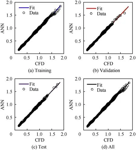
Fig.14.Regression of training samples, validation samples, testing samples.

Fig.15.Error histogram of different samples.

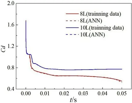
Fig.16.Comparisons between ANN prediction results and training data when σ =0.0215.

(1) The cavity will develop, fuse and collapse in the water and natural supercavitation phenomenon is observed when underwater serial projectiles move at a high speed.The serial multi-projectiles structure can reduce the drag of the second projectile and achieve the goal of drag reduction.

Fig.17.Comparisons between ANN prediction results and CFD computational results when σ = 0.0110.

(2) The length and aspect ratio of supercavity around serial projectiles decrease with the decreasing of the cavitation number, and the drag coefficient of the second projectile decreases.The length and aspect ratio of supercavity decrease with the decreasing of the distance between serial projectiles, and the drag coefficient of the second projectile decreases.

(3) The drag coefficient of the second projectile predicted from ANN model has a high accuracy, where the regression Rvalues of training, validation and testing samples are all above 0.99.Machine learning has an obvious advantage in simplifying computational complexity and increasing computational efficiency.

(4) Furthermore,the discussion of different cases is based on the static projectiles.However,in the real-world application,the movement of serial projectiles should be considered.This is the future direction for this work.

The authors declared that there is no conflict of interest.

This work is supported by the National Natural Science Foundation of China (Grant No.11972194,12072160).