Elastoplastic constitutive modeling under the complex loading driven by GRU and small-amount data

Zefeng Yu, Chenghng Hn, Hng Yng, Yu Wng, Shn Tng,b,c,*, Xu Guo,b,c,*

aThe State Key Laboratory of Structural Analysis for Industrial Equipment, Department of Engineering Mechanics, Dalian University of Technology, Dalian,116023, China

b International Research Center for Computational Mechanics, Dalian University of Technology, Dalian, 116023, China

c Ningbo Institute of Dalian University of Technology, Ningbo, 315016, China

Keywords:Data driven Recurrent neural network Path dependence Small-amount data

ABSTRACT In this paper, a data-driven method to model the three-dimensional engineering structure under the cyclic load with the one-dimensional stress-strain data is proposed. In this method, one-dimensional stress-strain data obtained under uniaxial load and different loading history is learned offline by gate recurrent unit (GRU) network. The learned constitutive model is embedded into the general finite element framework through data expansion from one dimension to three dimensions, which can perform stress updates under the three-dimensional setting. The proposed method is then adopted to drive numerical solutions of boundary value problems for engineering structures. Compared with direct numerical simulations using the J2 plasticity model, the stress-strain response of beam structure with elastoplastic materials under forward loading, reverse loading and cyclic loading were predicted accurately. Loading path dependent response of structure was captured and the effectiveness of the proposed method is verified. The shortcomings of the proposed method are also discussed.

Engineering structures often are subjected to a variety of load types. Some parts of them may experience a complex deformation history, for example, plastic deformation under cyclic loading. The materials of such structures often include nonlinearity and path (history) dependence. Appropriate nonlinear constitutive models considering loading path (history) can assist in structural design, help monitor structural health and assess the redundancy life of the engineering structures. Many constitutive models have been proposed to describe the behavior of elastoplastic materials [1–4] based on an explicit-functions-based paradigm with basic elements such as the plastic flow, loading and unloading judgment etc.. However, the formulation of function-based constitutive model along with the traditional approach is a challenging and time-consuming job. It requires complex mathematical derivation and intuition into the plastic deformation mechanisms of the materials. In recent years, with the development of the data-driven approach and the machine learning by the deep neural networks[5,6], building the constitutive models through the combination of data science and solid mechanics attracted the research attention of the researchers around the world.

With the development of data science in recent years, numerous data-driven approaches have been proposed to replace traditional constitutive models. Furukawa and Yagawa generalized the inelastic material behaviors as a state-space representation and proposed a one-dimensional viscoplastic constitutive model using artificial neural networks (ANN) in which the stress, viscoplastic strain and internal variables as input and plastic strain rate and rate of internal variable as output [7]. The one-dimensional mechanical response of the viscoplastic solder alloy subjected to strain rate jumps, temperature changes, or loading-unloading cycles is learned through the specifically designed long shortterm memory (LSTM) networks [8]. Zopf and Kaliske [9] proposed a model-free approach for the characterization of the uncured elastomer in a three-dimensional setting. Coupling with the microsphere approach, the neural networks only need to represent the stress-stretch dependence in one dimension. However, this approach did not consider the interaction between the one-dimensional states along with the different directions in the microsphere model. Mozaffar et al. [10] generated the stress-strain data along the different loading paths in two-dimensional space and the elastoplastic model is then built through the learning by recurrent neural network (RNN) based on the generated data. Similar studies have also been carried out [11–14]. Numerical simulations are often adopted to generate the data to train the neural networks in most of the above mentioned studies. It often requires a lot of data to obtain high-quality neural networks. For example,Mozaffar et al. [10] generated 15,000 samples with different loading series to obtain stress-strain data under different loading paths.With the huge amount of data to train the neural networks, the trained model represented by the neural networks usually includes a lot of parameters and internal variables in RNN. Then it is very hard to be implemented into the existing finite element software for further structural analysis.

Since uniaxial experiment is the most convenient way to obtain the stress-strain data, developing a computational model to predict the elastoplastic response under the three-dimensional setting and complex loading paths using only one-dimensional data is important. For engineering applications, successful implementation of the model into the finite element software is also essential. It requires that the trained model should be as compact with fewer parameters and internal variables as possible. Tang et al. [15]proposed the MAP123 method which realized the mapping from one-dimensional (1D) data to three-dimensional (3D) problems by the proposed coaxial relationship. MAP123-EP is also proposed to model the elastoplastic materials driven by the stress-strain data directly, avoiding the explicit function-based elastoplastic models[16]. Unfortunately, MAP123-EP cannot be applied to reverse loading and cyclic loading.

In this paper, MAP123-EP is further developed to model the response of engineering structures under the reverse and cyclic loading. The generated stress-strain data along different uniaxial loading paths is trained by GRU. The trained model is implemented into the finite element software for structural analysis. Compared with the reference model, the obtained material model can accurately predict the path and history dependent response of the three-dimensional beam under complex loading paths, e.g., forward loading, unloading, and reverse loading.

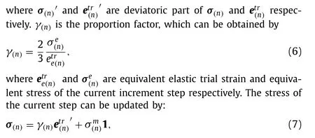
where 1 is 2-order identity tensor.

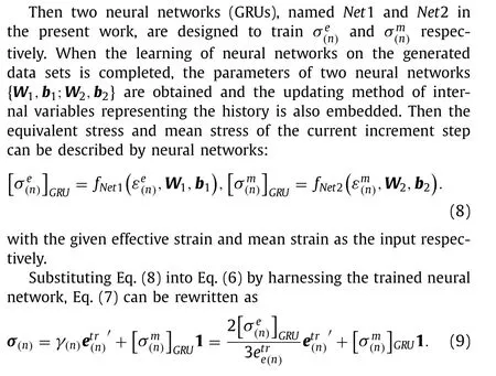
According to Tang et al. [15], it can be observed that the stresses can be updated with the known one-dimensional relationship between stress and strain for nonlinear elastic materials. However, for the elastoplastic materials, there is no one-to-one mapping between the stress and strain because this relationship depends on the loading history. With the development of new neural networks, GRU, one of them, may have the capability to obtain the stress as a function of strain in such cases with the internal variables embedded in the neural network. If we can generate the data set of 〈εe,σe〉 and 〈εm,σm〉 by one-dimensional experiments under different loading history, the GRU can be used to train the relationship between stress and strain. To make the training easier,σeandσmare assumed to be uncoupled. The data sets of 〈εe,σe〉and 〈εm,σm〉 are trained respectively. This assumption can help to reduce the amount of data for neural network training. It also can improve the stability of the application of neural networks in numerical simulations.

For three dimensional structure, if the strain of a material point is known at the current step, the stress (three-dimension) can be updated directly even under the history-dependent loading by proposed method. The judgment of the loading and unloading state of the material also can be avoided during the stress updating process.

After data preparation, postprocessing and network training, the neural network can be reformatted and programmed into the user material interface in any finite element software, e.g., UMAT in ABAQUS. This should be applied to the Gauss integration point of every element.

In order to train the neural networks which can describe the mechanical response of elastoplastic materials, one-dimensional stress-strain data should cover the typical loading history, such as loading and unloading, reverse loading, cyclic loading etc.. As an initial attempt, the numerical experiments are adopted to generate the required data. Then, in this paper, a 1 mm×1 mm×1 mm cell is used. The uniaxial displacement is loaded in thexdirection(Fig. 1a). The displacementu1is randomly generated by a method based on the Gaussian process [17]. A sample of the generated displacement vs. time is shown in Fig. 1b. 〈εe,σe〉 and 〈εm,σm〉 can be extracted from the output strain and stress. A total of 400 samples of displacement vs. time were generated and used for training.Each sample takes 200 data points.

Fig. 1. a A cell to generate a 1D stress-strain data by the randomly generated displacement load. b A sample of displacement load vs. time generated by the gaussian process. 400 samples are used to generate the stress-strain data to train GRU.

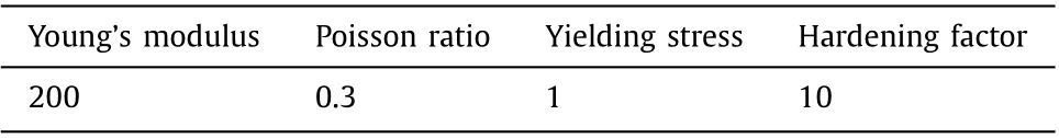
Table 1 Parameters of the reference J2 plasticity model (non-dimensional)

In this paper, J2 plasticity model, taken as the reference model,was chosen to generate the stress-strain data through numerical experiments. The yield function of the J2 plasticity model can be written as

Hereσfis flow stress, which is a function of accumulated effective plastic strain

whereσ0is initial yield stress,His the plastic modulus andqis the accumulated equivalent plastic strain. The parameters for the reference J2 plasticity model adopted in the present work are given in Table 1.

It should be noted that both uniaxial tension and compression experiment should be considered for data generation because the complex loading process may involve both compression and tension stress states.

GRU is adopted to represent the history dependent behavior of elastoplastic materials. A specific introduction to GRU can be found in Appendix A. The GRU training process in this paper is implemented using TensorFlow. Two neural networks are defined to train 〈εe,σe〉 and 〈εm,σm〉 respectively. It should be pointed out that the relationship between 〈εe,σe〉 is more complex for plasticity than that of 〈εm,σm〉. Therefore, a relatively simple network structure is adopted to learn the relationship between mean stress and mean strain to greatly reduce the parameters in the neural network. Among the 400 sets of the data under different loading paths, 360 sets are selected as training one, and the other 40 sets are used as test one. The initialization of networks (Net1 andNet2) weights and biases follow the default settings of TensorFlow.The learning rate is selected as 0.001, the batch size is 64, and the epoch is 3000. The optimization algorithm, commonly used Adam,is adopted. The loss function is the mean squared error of the normalized target value. The structures of the two neural networks and the final training errors after the normalization are shown in the Table 2, where GRU indicates the gated recurrent unit, and FCN indicates fully connected neurons.

The processor for solving the problems shown in this paper is Intel i9-10850K, and the GPU is NVIDIA RTX3060. The data generation time for 400 paths is 6089.80 s with 5 cores of the processor. The time cost used for network training onNet1 andNet2 are 1064.80 s, 526.24 s respectively.

We first verify that the learned plasticity model can reproduce the elastoplastic material behaviors under the complex loadings at the material level. A 1 mm×1 mm×1 mm cube (Same as the cell that generated the data) is built. Then the displacement load is applied to verify the accuracy of the trained constitutive model based on the proposed method to predict the mechanical responses.

Two cases are considered. Under the uniaxial tensile loading(case 1), thexdegree of freedom of the bottom surface (x=0) is fixed. The time-varying displacementu1of the surface is imposed on the top surface (x=1), see Fig. 2. Under the shear loading (case 2), the bottom-face of the cube (y=0) is fixed. The time-varying displacementu2along thex-direction is applied on the top-face(y=1), also see Fig. 2.

In both case 1 and case 2, the displacement vs. time imposed on the cube is totally different from those to generate the stressstrain data for model training. However, as shown in Fig. 3, stress componentσ11vs. time predicted by the trained model agrees with that generated by the reference J2 plasticity model. Both the elastic stage before entering into the plasticity and the plastic stage with lower instantaneous modulus can be observed. The hardening as a function of the accumulation of the plastic deformation is also learned successfully. It should be emphasized again that the present trained model for online computation does not involve the judgment of loading and unloading directly, unlike the finite element simulation with the traditional J2 plasticity model. It is concluded that the proposed method in this paper can accurately predict the history and path dependence of elastoplastic materials. For the shear case 2, a comparison of the Mises stress vs. time predicted by the trained model with that generated by the reference J2 plasticity model is also shown in Fig. 3. The results calculated by both models agree with each other very well. The same conclusion can be drawn as the case 1. The time-cost comparison for online computation between the traditional J2 plasticity model and the trained model is given in Table 3. Furthermore, the trained material model is used to predict the mechanical response of the engineering structure. A three-dimensional beam with length of 20 mm, width of 4 mm and height of 5 mm is used, shown in Fig. 4a.The units of length and displacement are mm. Thexdegrees of freedom of the bottom surfacex=0 is fixed and a time-varying displacementualong thez-direction is imposed on the top surface (see Fig. 4b). Both J2 plasticity model and the present trained model are employed to describe the elastoplastic material behaviors respectively. Finite element simulations are carried out and the entire loading process ofuis equally divided into 40 incremental steps in the simulations by the J2 plasticity model. And a total of 50 incremental steps were used in the trained model simulation.

A comparison of the predicted contours of Mises stress by both models has been shown in Fig. 4c at times 1 s, 2.5 s, and 4 s.The average relative errors of Mises stress of the three time moments are 4.94%, 8.47%, and 4.87%, respectively. Results predicted by the trained model agree with those by the J2 plasticity model well. It indicated that the trained model can be embedded into the finite element software and can be used for structural analysis with elastoplastic material. At present, small step is required for the structural analysis with multiple elements. Online computational time cost with the J2 plasticity model is 24s but approximately an hour with the trained model. However, the present work pays more attention to the computational method and less on time efficiency. As we know, it is difficult to predict the history dependent material behavior efficiently, faced by the data-driven computational mechanics community. We will try to incorporate the known physical symmetry to overcome the efficiency issue in our future research.

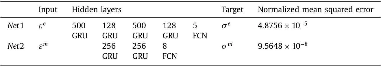
Table 2 Two networks for training of the mechanical response

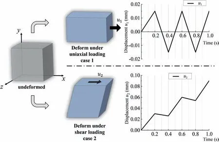
Fig. 2. A 1 mm×1 mm×1 mm cube is subjected to the uniaxial and shear loadings respectively (case 1 and case 2), which are used to verify the present trained model.

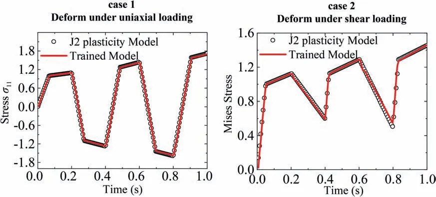
Fig. 3. Comparison of predictions by the reference J2 plasticity model and the present trained model for case 1 and case 2 respectively.

This paper proposed a data-driven method to model the elastoplastic behavior of the three-dimensional structure under the cyclic load with the one-dimensional stress-strain data. Compared with traditional finite element analysis with the function-based constitutive models for elastoplastic materials, the proposed method can describe loading path dependent elastoplastic behavior without knowing the explicit function form of the material model. Moreover, unlike the most established data-driven method (for example, Mozaffar et al. [10]), it avoids the usage of the stress-strain data under complex stress states and loading paths. The proposed method can use only a small-amount of 1D stress-strain data to predict the elastoplastic behavior successfully in the 3D stress state under complex loadings. Furthermore, the trained model can be embedded into the finite element analysis software to predict the mechanical response of the engineering structure. The present method needs further improvement. In the future, the known physical symmetry should be incorporated, to promote its application to predict the complex elastoplastic behaviors.

Fig. 4. a Geometric model of the three-dimensional beam for the comparison of the trained model and reference J2 plasticity model. b Displacement loading vs. time imposed on the right end surface of the beam. c The equivalent stress contour of the beam at the different time moments predicted by the trained model and the reference J2 plasticity model.

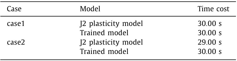
Table 3 Comparison of the online computational time cost by the traditional J2 plasticity model and the trained model

Declaration of Competing Interest

The authors declare that they have no known competing financial interests or personal relationships that could have appeared to influence the work reported in this paper.

Acknowledgments

The support of the Project MKF20210033 is acknowledged.

Appendix A. Introduction to the GRU architecture

GRU is a variant of RNN, proposed to solve problems in RNN such as long-term memory and vanishing gradients in backpropagation. GRU can better capture the dependence on larger time step in the time sequence. For GRU, the hidden statehcan convey past relevant information in the time sequence. At each time step, the hidden state in the GRU cell is updated according to the hidden state of the previous time step and the input of the current time step. Figure A1 shows the core structure of GRU, composed of the reset gate and update gate, which can process the historical information in each GRU cell to update the hidden stateh.

rtis reset gate, which controls how the hidden stateht−1of the previous time step flows into the candidate hidden statehtof the current time step. In other words, the reset gate determines what information about the previous hidden stateht−1is forgotten.ztis update gate, which controls how the hidden state should be updated by the candidate hidden statentcontaining the current time step information. In other words, the rest gate and update gate decide what information to throw away and what to keep.When the reset gate approaches 0, the hidden state is forced to ignore the hidden state of the previous step.rtandztare updated as follows:

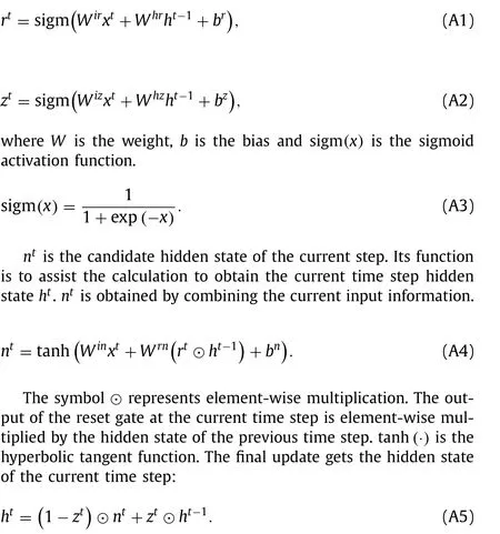
In practical applications, one layer usually containsmGRU cells,and the hidden state of each layer is an m-dimensional vector. It is generally followed by a fully connected neural network to realize the learning of the hidden state to the output target value.

Fig. A1.Time series processing of GRU cell and internal structure consisting of reset gate and update gate.