Inter-Annual Variabilities of the Body Weights of Two Cephalopod Species in the Yellow Sea Under Different Environmental Conditions
2022-02-24GUOJianzhongZHANGChiLIJianchaoTIANYongjunYEZhenjiangLIZhixinandGAOZihui
GUO Jianzhong, ZHANG Chi, LI Jianchao, TIAN Yongjun, 2), 3), 4), *,YE Zhenjiang, LI Zhixin, and GAO Zihui
Inter-Annual Variabilities of the Body Weights of Two Cephalopod Species in the Yellow Sea Under Different Environmental Conditions
GUO Jianzhong1), #, ZHANG Chi1), #, LI Jianchao1), TIAN Yongjun1), 2), 3), 4), *,YE Zhenjiang1), LI Zhixin1), and GAO Zihui1)
1),,266003,2),,266100,3),,266071,4),,,266003,
As fish stocks have been overexploited and catches have decreased over the last few years, the cephalopod catch has increased globally to the point that they are now among the most important marine resources in the world. Climate change and human activities greatly affect the growth and abundance of cephalopods. Understanding how the individual growth of key species varies and how they respond to environmental changes is essential for an effective fishery management.andare two dominant species in the cephalopod community of Yellow Sea (YS).Both of them are commercially important and have great ecological values. Herein, we compared the body weights () of these two species from 2011 to 2018 based on an analysis of biological parameters (., mantle length and) from trawl surveys in the YS. Considerable temporal variations in theof the two species are apparent. Specifically, theofwas the lowest in 2011 and the highest in 2017, andthe well growth was noted in 2015–2018. Theofwas the lowest in 2013 and the highest in 2016,while well growth was observed in 2015–2016. Mixed-effect models indicate that theof these species correlates significantly with the sea surface temperature (SST) and Southern Oscillation Index (SOI), suggesting the impact of the regional environment associated with strong ENSO events on. In a different response window, growth increases with increased SST and decreases with increased SOI. The consistent patterns of theof these cephalopods in response to environmental factors demonstrate they can be employed as indicator species for studying environmental change in the YS. Our results improve the understanding of the responses of cephalopods to environmental changes in the YS, as well as the mechanisms that drive their growth. Such information is critical for the effective management and sustainable development of cephalopod fisheries in this region.
;; body weight; environmental changes; Yellow Sea
1 Introduction
Cephalopods (., squid, octopod, and cuttlefish) are a major component of global marine ecosystems (Chesnais., 2019). A wide variety of species representing im- portant components of the local ecosystem (Clarke, 1996; Xavier., 2014) inhabit coastal and shelf waters, which are characterized by high primary and secondary produc- tivities (Longhurst., 1995). Cephalopods in coastal and oceanic areas have recently increased in abundance in response to changing ocean environments (Doubleday., 2016; Pang., 2018). Ce phalopods are charac- terized by rapid growth, a short lifespan, high turnover rates, and strong phenotypic plasticity (Pecl and Jackson, 2008; Arkhipkin., 2021). Their flexible life strategies render them capable of quick responses to changing envi- ronments. Researchers believe that cephalopods mayeven- tually overtake fish species in coastal ecosystems, which have become degraded as a consequence of fishing pres- sure and climate change (Pierce., 2008; Doubleday., 2016).
China’s seas, which are among the largest marine eco- systems in the world, have demonstrated rapid warming with climate change (Pang., 2018). For example, sea surface temperatures (SSTs) in the East China Sea have risen by 1.22℃ from 1982 to 2006 (Belkin, 2009); in the Yellow Sea (YS), the SST has increased by 1.7℃ since 1980 (Lin., 2005; Pei., 2017). China’s seas are overexploited, and commercial fish landings have decreased significantly; interestingly, however, cephalopod landings have increased (Pang., 2018). The YS is a semi-en- closed marginal sea located in the Northwest Pacific Ocean, surrounded by the Korean Peninsula and mainland China. The area of this sea is approximately 380000km2, and its average depth is approximately 44m (Park., 2015). The YS is an intensively exploited shallow sea ecosystem (Wang., 2016) and an important global resource for coastal and offshore fisheries (Tang, 2003). Climate change, overfishing, and exploitation have affected the self-regu- lating mechanism of the YS ecosystem (Tang, 2003). Indeed, 90% of its fishery resources are now in danger of exhaustion change (Jin, 2017), which could alter its com- munity structure (Lin., 2005; Wang., 2016). De- spite this situation, the cephalopod catch in this region hasincreased since 2003, stabilizing at approximately 10×104t from 2003 to 2013 (Wang., 2016). Chlorophyll(Chl-) concentrations have also trended upward since 1998 (Tan., 2011; Tian., 2020).
The cephalopod fauna of the YS mainlycomprises 14 warm-temperate speciesbelonging to six families.The do- minant taxa areand(mainlyand), followed by(Du., 2016).andare the primary catch spe- cies of cephalopod fisheries, and they are commercially and ecologically important throughout the whole China’s waters (Dong, 1978; Du., 2016; Jin., 2017). For example, thecatch in early spring of 1970s was 85% of the annual cephalopod catch in China (Dong, 2014). Both species live in shallow coastal waters and have life cycles of less than one year. The loliginidper- forms diel migrations in surface waters at night, while post-paralarvais basically benthic (Dong, 1988; Jin., 2020; Pang., 2020). Both species are highly sensitive to environmental changes, which renders them of potential value in monitoring exercises to detect environ- mental change (Pecl and Jackson, 2008; Chesnais., 2019). As one species is a squid and the other is an octo- pus, they also likely reflect different responses to environ- mental changes. Research on these taxa has focused on molecular genetic analysis (Jiang., 2015; Um., 2017). Unfortunately, the lack of basic biological informa- tion on these species limits our acquisition of a compre- hensive understanding of their population dynamics.
Condition factors are important for evaluating the health of aquatic species, populations, and communities (LeCren, 1951; Ferreri, 2014). They can be affected by an indivi- dual’s size, sex, sexual cycle, food supply, and habitat (Mo- hapatra., 2010; Zhang., 2017). Without specific age data, condition factors have indicated biochemical,ecological, and physiological processes in studies on the phenotypic responses of fish (Maina., 2019), crab (Zhang., 2017), shrimp (Ramírez and Paramo, 2020), and cephalopods (Ferreri, 2014; Siddique., 2014) to environmental change. Growth integrates the effects of physical and biological processes and is an ideal parame- ter for measuring the response of organisms to environ-mental change and fishing pressure (Morrongiello., 2012).
The scarcity of information on the population dynamics of cephalopods in the YS hinders our understanding of how cephalopods have already responded and will respond to changes in the marine environment. In this study, we in- vestigate the appropriateness ofandas indicator species fordetecting environmental change by comparing inter-annual variations in theirbody weight ().We use a mixed-effects model to analyze the weight growth of these two species responding to environmental factors with the goals of 1) reproducing inter-annual variations infor both species, and 2) analyzing environmental fac- tors on the weight growth of each species.
2 Materials and Methods
2.1 Sampling Survey
Squid and octopus samples were collected from bottom trawl surveys in the YS during the spring (May) and au- tumn (September) of 2011 and 2013–2018 (Fig.1). The survey vessel was a 220kW single tugboat that was car- ried out during the day with a towing speed of 2–3 knots per hour at each station. We determined the water depth at each station through measurements of conductivity, temperature, and depth profiler and recorded each tow. The sur- vey water depth ranged from 10m to 75m, and the aver- age water depth was 35.2m. Species were identified fol- lowing Dong (1988) and Okutani (2015). The dorsal man- tle length (, mm) and(0.1g) of 4192and 1100individuals (representing 66.21% and 19.32% of the total cephalopod catch, respectively; Table 1) were measured.
2.2 Marine Environmental Data
SST and Chl-are oceanographic variables that are con- sidered most suitable for determining cephalopod habitat (Arkhipkin., 2015). The Southern Oscillation Index (SOI) was used as an important climate index in the Paci- fic (Power and Kociuba, 2011). SOI is significantly nega- tively correlated with the average SST in the YS and af- fects the intensity of the YS warm current, thereby impact- ing the YS ecosystem (Yin., 2016). We selected SST, Chl-, and SOI as environmental variables to study the ef- fects of their change on theofandover time. Data for each species from 2010 to 2018 were sourced as follows. (a) Monthly average SST and Chl-data (119˚–124˚E, 34˚–37.5˚N) were derived from the MODIS (Moderate-Resolution Imaging Spectroradi- ometer) Aqua products of the National Oceanic and At- mospheric Administration (NOAA) (https://coastwatch.pfeg. noaa.gov/). (b) Monthly average SOI data were derived from the NOAA (https://psl.noaa.gov/gcos_wgsp/Time series/Data/soi.long.data).Here, the annual average SST and Chl-are represented by the annual average of their corresponding monthly averages (±SE). The spatial reso- lution of all marine environmental data is 0.1˚.
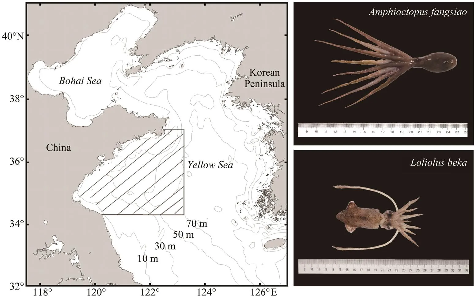
Fig.1 Sampling area (hatching region) of representative Amphioctopus fangsiao (upper) and Loliolus beka (lower) specimens.

Table 1 Sample data for Loliolus beka and Amphioctopus fangsiao
2.3 Statistical Analysis and Model Building
is used to evaluate the condition factors ofand. Regression and correlation analyses were performed betweenand, and a one-way analysis of variance was used to identify differences in weight growthamong years. A least-squares method was used to test length-weight relationships (LWR) for both species with following equation (LeCren, 1951):
, (1)
whererepresents the individual’s nutritional status, andrepresents its growth pattern. Because the variance ofincreases asincreases, the above equation was log- transformed to:

We fitted a generalized linear model (GLM), a simple linear model suitable for individuals at different years and water depths (forand, respectively), and two linear mixed-effect models (LMEM) considering the year and/or depth as random factors to explain the re- lationship betweenand(Ma., 2017). All mo- dels forincluded the maximum intrinsic fixed effect structure. Akaike’s information criterion for small sample size (AICc) was used to evaluate the relative support of each candidate set in the model, which was further correct- ed for the small sample size, to determine the optimal growth model (Beier., 2001) (Table 2).

Table 2 Models to assess the length-weight relationships of Loliolus beka and Amphioctopus fangsiao
Sliding window analysis was performed on the basis of the growth model to determine the optimal time window for weight growth to occur in response to environmental variables (Van de Pol., 2016). This type of analysis can test the influence of different environmental variables on the response variables in different time windows and compare different time windows to determine which en-vironmental variables can best predict biological responses(Smoliński, 2019b). Absolute time windows and linear and quadratic relationships were assumed in the analysis. In addition, 1000 randomization tests were performed to eli- minate the possible misclassification of environmental sig- nals due to change (., false positives) (Smoliński, 2019a). The possibility of obtaining a powerful model supported by chance was quantified by calculating the∆AICcvalue from 1000 randomized trials. The sliding window analysisindependently considers the external effects of SST, Chl-, and SOI as fixed effects within a certain time window. The AICc and significance tests were used to determine the best model, and restricted maximum likelihood esti- mation was used for refitting to obtain unbiased variable estimates (Zuur., 2010). The predicted effect-value shows the degree of correlation between environmental variables and, and thevalue represents the sequen- tial-test analysis (STARS) results of the obtained time series toidentify significant step changes in. All ana- lyses were performed using the R Studio 3.5; ‘lme4’ was used for building mixed models;‘MuMIn’ was used to cal- culate conditional2-values;‘AICcmodavg’ was used to calculate AICc; and ‘climwin’ was used to obtain the slid- ing window to predict which environmental variables af- fect weight growth the most.
3 Results
3.1 Mantle Length and Body Weight Distribution
Inter-annual changes in the frequency distributions ofandin spring and autumn are apparent forand(Fig.2). Thedistributions of both species in autumn are generally unimodal (mainly between 30 and 40mm for,and between 40 and 50mm for), whereasdistributions during spring are more scat- tered. Thedistribution ofis concentrated be- tween 0 and 5g in spring and autumn, whereas that ofis relatively dispersed in the same seasons. The range and mean of theofin spring are high- er than those in autumn.
3.2 Length-Weight Relationship
The LWR relationships (as Eq. (1)) ofanddiffer seasonally (Fig.3).
For,
,
.
For,
,
.
Whereas the allometric coefficientfor each species is the largest in spring,is the largest in autumn. In general,andvalues in autumn are lower than those in spring, which indicates that spring environments are more condu- cive to growth.
3.3 Inter-Annual Changes in Weight Growth
AICc values indicate that LMEM with year and depth and random effects on the intercept is the best model (Ta- ble 2) among those tested, thus reflecting the impact of en- vironmental differences in the habitat depth of these two species on their.models forandrespectively explain 73.80% and 75.26% of the vari- ance noted for each species, and the 7-year weight growths ofandare reconstructed based on the growth model. Theof each species varies greatly among different years, and the trends observed vary between spe- cies (Fig.4). Theofmanifests an overall up- ward trend, especially after 2014, and peaks in 2017. Theoffluctuates remarkably and is the lowest in 2013,and the highest in 2016. Obvious seasonal diffe- rences in intraspecificpatterns are apparent (Fig.5). Themaximum peak foroccurs in spring and autumn of 2016, while that foroccurs in spring of 2017.The growth trends gradually increase from autumn of 2011. Both annual (Fig.4) and seasonal (Fig.5)changes show obvious annual variations. The ‘year’ factor plays a key role in understanding the long-term seriesof the two species, while the ‘season’ factor exerts a local effect on the current year.
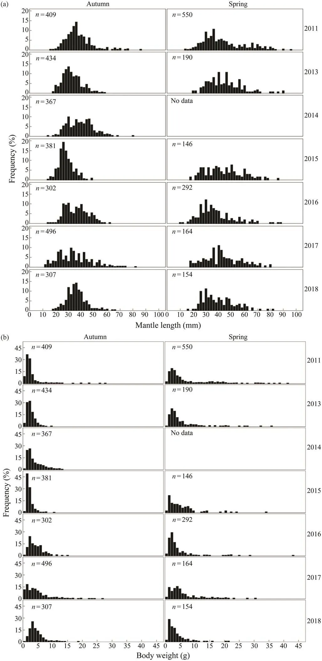
Fig.2 (a), (b) Inter-annual variations in the ML and BW frequency distributions of Loliolus beka in spring and autumn.
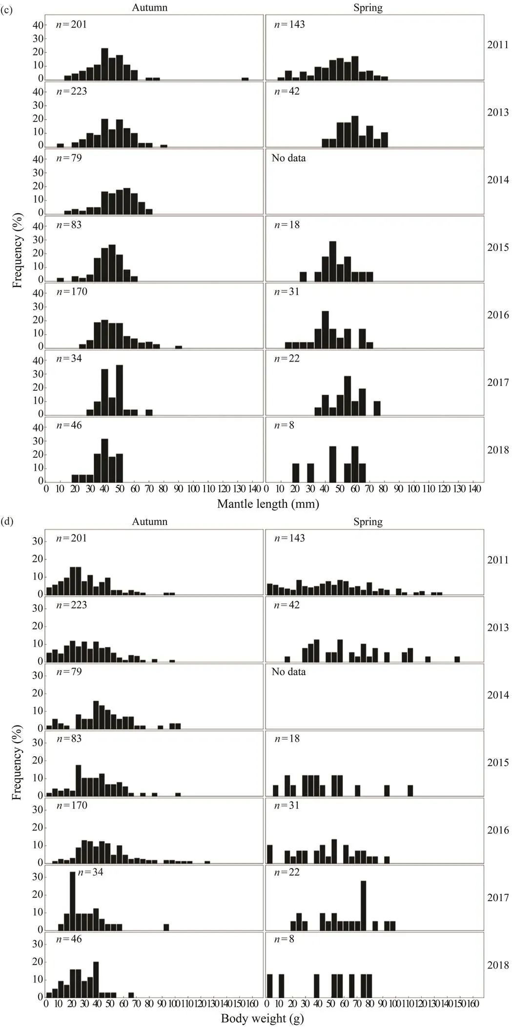
Fig.2 (c), (d) Inter-annual variations in the ML and BW frequency distributions of Amphioctopus fangsiao in spring and autumn.
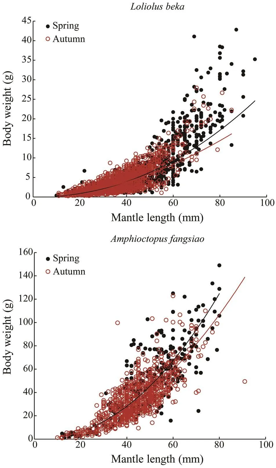
Fig.3 Seasonal relationship between ML and BW for Loli- olus beka and Amphioctopus fangsiao. The curves repre- sent seasonal power regressions for the relationships be- tween ML and BW (black, spring; red, autumn).
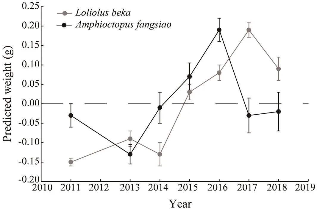
Fig.4 Inter-annual variations in BW based on yearly random- effect estimates (±SE) for Loliolus beka and Amphioctopus fangsiao.
3.4 Inter-Annual Variations in Environmental Factors
Inter-annual variations in SST, Chl-, and SOI are shown in Fig.6. SST increases from 13.8℃ in 2011 to 16.6℃ in 2016, and then to 16.8℃ in 2017. Chl-trends downward from 2014 (2.8mgm−3) and is the lowest in 2018 (2.0mgm−3). SOI decreases from 2011 to 2015, increases from 2015, and peaks in 2011 (1.4).The lowest SOIs are noted in 2015 (−1.2) and 2016 (−0.5).
Fig.5 Inter-annual variations in BWby season based on year-ly random-effect estimates (±SE) for Loliolus beka and Am- phioctopus fangsiao.
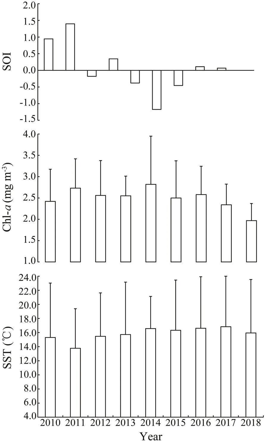
Fig.6 Inter-annual variations in SST, Chl-a, and SOI in the Yellow Sea, 2010–2018.
3.5 Environmental Effects on Body Weight
Sliding window analysis was used to identify the opti- mal time window for each environmental variable (Table 3; Figs.7, 8). The inclusion of these variables improves the model fitness and is supported by the AICc comparisons (Figs.7, 8). The ΔAICc value of the best model fitted to the observed data was compared with that of the null modelto obtain the optimal opening and closing time window pe-riods, and the environmental variables all reveal strong sig-nals (red areas in Figs.7, 8). Theresponse of both spe- cies is significantly related to SST and SOI, and the∆AICcobtained from the randomization test is <0.001. These re- sults suggest that SST and SOI signals are very unlikely to be false positives. In a different response window,increases with increasing SST and decreases with increas- ing SOI (Figs.9, 10).also responds significantly to Chl-, and the∆AICcdetermined from the randomization test is <0.001. This value indicates that the signal is un- likely to be a false positive (Fig.9).

Table 3 Predicted effect of significant environmental predictors on BW (–, not available)

Fig.7 Optimal window identification of environmental variables for Loliolus beka ((a), SST; (b), Chl-a; (c), SOI). Months for which windows are open and closed are shown on the y and x axes, respectively. ΔAICc (indicated by the gradient) reflects differences of BWs with environmental variables.
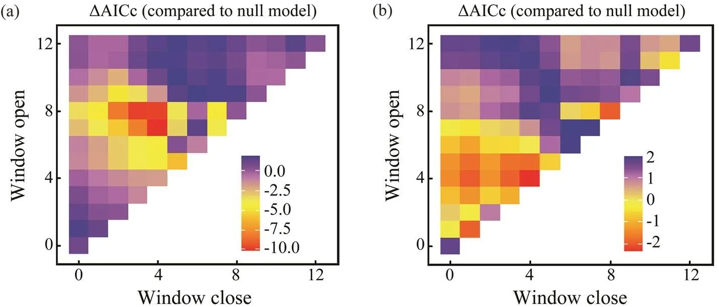
Fig.8 Optimal window identification of environmental variables for Amphioctopus fangsiao ((a), SST; (b), SOI). Months for which windows are open and closed are shown on the y and x axes, respectively. ΔAICc (indicated by the gradient) re- flects differences of BWs with environmental variables.

Fig.9 Predicted effects of SST, Chl-a, and SOI on the BW of Loliolus beka. The gray dotted line represents the 95% con- fidence interval, and the solid black line represents the fitting relationship between environmental factors and BW.
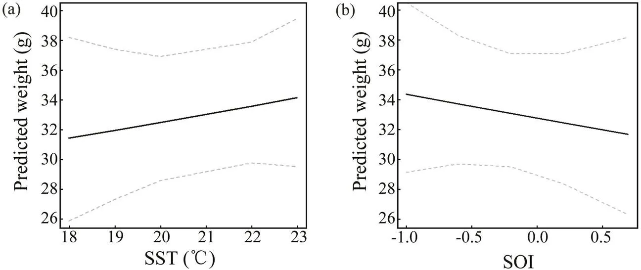
Fig.10 Predicted effects of SST and SOI on the BW of Amphioctopus fangsiao. The gray dotted line represents the 95% confidence interval, and the solid black line represents the fitting relationship between environmental factors and BW.
4 Discussion
Because of rapid warming and overexploitation of Chi- na’s seas, the YS ecosystem has degraded, and high-tro- phic level species have decreased (Tang, 2003). However, the abundance of cephalopods has increased, most likely because of their significant phenotypic plasticity and re- duction in the number of predators (Wang., 2016;Arkhipkin., 2021).andoccupy relatively high trophic levels and feed mainly on benthic crustaceans and small fish larvae (Huang, 2004; FAO, 2010).These two species have come to occupy dominant positions in the YS ecosystem (Du., 2016).
4.1 Growth Characteristics
The developments of cephalopods differ as a result of differences in their life history, gonad development, food supplies, and habitats (Semmens., 2004; Pecl and Jack- son, 2008; Pang., 2020). We found that theofandvaries remarkably over time, and thetrends for each species differ (Fig.4) according to their uni- que life histories (Dong, 1988). Obvious seasonal differ- ences in the growth of the same species can be observed (Fig.5), which is closely related to their changing life his- tory characteristics at different developmental stages andseasonality in their habitat (Semmens., 2004; Pecl andJackson, 2008). The number of individuals of each spe- cies caught in spring is lower than that in autumn (Table 1), which may be related to fishery seasonality (Jin., 2020). The spawning population ofis mainly tar- geted in spring, and lower catches are often obtained in this season; individuals weighing <5g account for 69.45% of the total catch in this season (Fig.2).is mainly obtained in early spring when it begins to spawn; the catchduring this season is usually smaller than that in other sea- sons.
We could only investigate seasonal differences in LWR because many individuals in the samples were unsexed (Fig.3). LWR differs between species and seasonally with- in a species, as mainly reflected by parametersand(Fig.3). Because the LWRvalues of the two species are <3, their weight growth follows an allometric growth pat- tern. Moreover, thevalues of both species are greater in spring than those in autumn, indicating greater springs. This finding is supported by the data in Table 1.The num- bers and weights of individuals of>60mm in spring are greater than those in autumn (Fig.3), which could berelated to overfishing after the closure of the summer fish- ing closure season. The LWR2values for each species are relatively low because growth is susceptible to changes in environmental conditions (Semmens., 2004). This re- sult is consistent with other studies on octopus species (Silva., 2002; Otero., 2007; Pang., 2020). Previous studies showed thatmainly spawns in spring (Dong, 2014), but the spawning season of the spe-cies may actually range from early spring to late autumn (Pang., 2020). A few of studies have reported the growth of. Large variations inandare also noted between individuals in the same season (Table 1, Fig.3), which may be caused by different developmental stages and age structures, as well as other factors. Further researches combining age determination and growth pat- tern analysis are recommendedon both species.
4.2 Effects of Environmental Factors on Growth
Temperature affects the aggregation, reproduction, mi- gration, growth, abundance, and population dynamics of cephalopods (Arkhipkin., 2015; Angeles-Gonzalez., 2017).anddemonstrate a posi- tive linear growth-SST relationship (Figs.9, 10) and simi- larpatterns from 2014–2016 and during spring (Figs.4, 5). Similar positive linear respond patterns have been observed in,,,(Forsythe, 2004; Keller., 2017; Sasi- kumar., 2018). Both species inhabit shallow waters, where temperature can synchronize life history features in seasonal habitats (Quetglas., 2011). In addition, the patterns of change in the inter-annualofrough- ly mirror those of SST (Figs.4, 6).is the highest in 2017and the lowest in 2011 (Fig.4), mainly because warmer waters support higher metabolic rates and higher food in- take (Semmens., 2004). Compared with the results of other studies in the past 20 years, cephalopods in the YS appear to have migrated further north because of warmer temperatures (Jin., 2020). Moreover, key window pe- riods forandgrowths occur in June and May–August (Table 3) when temperaturesare 14.9–22.6℃ and 17.5–23.4℃, respectively. These temperatures differ from those reported in previous studies (Jin., 2020), possibly because of differences in seasonal habitats. Further research is needed to examine the impacts of cli- mate change on seasonal species to predict changes in the YS ecosystem.
Chl-strongly influences prey density, habitat suitabi- lity, catch per unit effort (CPUE), and cephalopod abun- dance (Puerta., 2015; Keller., 2017; Yu., 2018). We observed a strong negative correlation betweenweight and Chl(Fig.9), possibly becauseperforms diel migrations near the seabed during the day and near the surface at night. By contrast,is a benthic species, and its response to Chl-is delayed by se- veral months (Dong, 1988; Puerta., 2015; Jin.,2020). Inter-annual variations intrend in theopposite direction to those of Chl-in our study. WhileChl-trends upward from 2011 to 2014 and downwardfrom 2014 to 2018 (Fig.6), theofis poor from 2011–2014 and improves after 2014 (Fig.4). Chl-in the corresponding critical window (mainly during winter and spring) is in the high-value during the year (Tian.,2020), but theofis poor, which may be re- lated to interspecies competition (Puerta., 2015; Kel- ler., 2017). Because small pelagic fishes effectively compete for food with early and juvenile stages of, higher Chl-may promote the growth of the former, there- by reducing the prey biomass for, which leads to its reduced weight (Keller., 2017). However, the ne- gative correlation between Chl-and growth may also be related to the growth rate. Higher primary productivity can accelerate development, thereby hastening sexual maturity at a smaller body size (Semmens., 2004). The Chl-range (2.4–3.4mgm−3) in this critical window is withinthe appropriate range (2.3–3.76mgm−3) reported in pre- vious studies, but the relationship between Chl-andis contradictory (Jin., 2020). This observation may be related to habitat seasonality and reflects the impact of environmental changes on species adaptability.
Climate change affects the growth, reproduction, and be- havior of cephalopods, especially during the El Niño-Sou- thern Oscillation (ENSO) (Yu., 2018). ENSO events, especially the SST anomaly and intensity of warm currentsin winter, affect SST by changing the surface heat flux with- in the YS; the strength of the main flow of the warm cur- rent has a lag relationship with the SOI (Wang., 2020). We found that theand SOI of these two species have a significant negative linear relationship, with the sliding window in the El Niño period exerting a delayed effect on growth, consistent with previous studies (Chen., 2007;Yu., 2018; Wang., 2020).The consistent re- sponse of theof the studied species to the SOI con- firms that ENSO can synchronize aspects of the life his- tories of a wide range of taxa over large geographic scales (Black., 2018; Tanner., 2020). El Niño and La Niña events affect the biological and physical environments, such as the hatching and feeding conditions of spawning grounds, thereby potentially affecting the number and growth of individuals likely to recruit into subsequent po- pulations (Chen., 2007). Because El Niño was strong during 2015–2016, temperatures in the YS increased, and theofandincreased. By contrast, 2011 was a La Niña year, and the lower temperatures in the YS were not conducive to theof both species (Figs.4, 6). Studies have shown that the spring and autumn CPUE ofin Haizhou Bay may be significantly nega- tively correlated with temperature during El Niño periods (Pang., 2020). ENSO events also affect other fish and zooplankton communities in the YS (Liu., 2020; Shi., 2020). For example, increased SST caused the win- tering grounds of Japanese anchovy () in the central and southern YS move northward (Liu., 2020).Therefore, ENSO modifies the YS environment and impacts the ecosystems of this area.
5 Conclusions
In conclusion, we examined inter-annual changes in theofandin the YS and used sliding window analysis and mixed-effects models to determine the impact of environmental factors on theof both spe-cies. We identified obvious inter-annual changes in theof both species. Relatively rapid environmental changes in the YS, especially SST and SOI, were reflected in theof both species, thereby indicating the impacts of the re- gional environment associated with basin-scale climate change, such as ENSO events. SST and SOI were consis- tently significantly correlated withbetween species, which indicates thatandcan be appro- priate indicators of environmental change in the YS. Ad- ditionally, Chl-concentration was strongly negatively cor- related with theof, possibly because of inter- species competition and growth rate variations. Climate change affects the catch environment, growth, and fluctu- ations of cephalopod populations in the YS.Knowledge of the long-term patterns of theofandand their consistent response to environmental vari- ables contribute to our understanding of how climate change affects cephalopod populations in the YS.
Acknowledgements
This research was supported by the National Natural Science Foundation of China (Nos. 41930534 and 41861 134037).
Angeles-Gonzalez, L. E., Calva, R., Santos-Valencia, J., Avila-Poveda, O. H., Olivares, A., Diaz, F.,., 2017. Temperature modulates spatio-temporal variability of the functional repro- ductive maturation of(Cephalopoda) on the shelf of the Yucatan Peninsula, Mexico., 83(3): 280-288, DOI: 10.1093/mollus/eyx013.
Arkhipkin, A. I., Hendrickson, L. C., Paya, L., Pierce, G. J., Roa-Ureta, R. H., Robin, J. P.,., 2021. Stock assessment and management of cephalopods: Advances and challenges for short-lived fishery resources.,78 (2): 714-730, DOI: 10.1093/icesjms/fsaa038.
Arkhipkin, A. I., Rodhouse, P. G. K., Pierce, G. J., Sauer, W., Sa- kai, M., Allcock, L.,., 2015. World squid fisheries., 23(2): 92-252, DOI: 10.1080/23308249.2015.1026226.
Beier, P., Burnham, K. P., and Anderson, D. R., 2001. Model se-lection and inference: A practical information-theoretic ap-proach., 65(3): 606-608, DOI: 10.2307/3803117.
Belkin, I. M., 2009. Rapid warming of large marine ecosystems., 81(1-4): 207-213, DOI: 10.1016/j.pocean.2009.04.011.
Black, B. A., van der Sleen, P., Di Lorenzo, E., Griffin, D., Sy- deman, W. J., Dunham, J. B.,., 2018. Rising synchrony controls western North American ecosystems., 24(6): 2305-2314, DOI: 10.1111/gcb.14128.
Chen, X. J., Zhao, X. H., and Chen, Y., 2007. Influence of El Niño/La Niña on the western winter-spring cohort of neon flying squid () in the northwestern Pacific Ocean., 64(6): 1152-1160.
Chesnais, T. D. L., Fulton, E. A., Tracey, S. R., and Pecl, G. T., 2019. The ecological role of cephalopods and their represen- tation in ecosystem models., 29(2): 313-334, DOI: 10.1007/s11160-019-09554-2.
Clarke, M. R., 1996. Cephalopods as prey. III Cetaceans., 351(1343): 1053-1065, DOI: 10.1098/rstb.1996.0093.
Dong, G., 2014.The basic biological studies on the artificial re- production of. Master thesis. Ocean Uni-versity of China (in Chinese with English abstract).
Dong, Z. Z., 1978. On the geographical distribution of the ce- phalopods in the Chinese waters., 9(1): 108-118 (in Chinese with English abstract).
Dong, Z. Z., 1988.. Science Press, Beijing, 90pp (in Chinese).
Doubleday, Z. A., Prowse, T. A., Arkhipkin, A., Pierce, G. J., Sem-mens, J., Steer, M.,., 2016. Global proliferation of cepha- lopods., 26(10): 406-407, DOI: 10.1016/j.cub.2016.04.002.
Du, T. F., Li, A., Dai, F. Q., Li, D., Liu, S. F., and Zhuang, Z. M.,2016. Survey and analysis of the autumnal cephalopod distri- bution in the Yellow Sea during 2006–2013., 23(4): 955-964, DOI: 10.3724/sp.j.1118.2016.15381 (in Chinese with English abstract).
FAO, 2010... Food and Agriculture Organization of the United Nations, Rome, 76pp.
Ferreri, G. A. B., 2014. Length-weight relationships and condi- tion factors of the Humboldt squid () from the Gulf of California and the Pacific Ocean., 33(3): 769-780, DOI: 10.2983/035.033.0311.
Forsythe, J. W., 2004. Accounting for the effect of temperature on squid growth in nature: From hypothesis to practice., 55(4): 331-339, DOI:10.1071/MF03146.
Huang, M. Z., 2004. Study on feeding habits and nutrient level of four cephalopod species from Taiwan Strait and its adjacent areas., 23(3): 331-340(in Chinese with English abstract).
Jiang, L., Wu, C., Liu, W., and Chen, M., 2015. Complete mito- chondrial genome of the., 27(6): 4278-4279, DOI: 10.3109/19401736.2015.1082093.
Jin, Y., Jin, X. S., Gorfine, H., Wu, Q., and Shan, X. J., 2020. Mo-deling the oceanographic impacts on the spatial distribution of common cephalopods during autumn in the Yellow Sea., 7: 1-17, DOI: 10.3389/fmars.2020.00432.
Jin, Y., Liu, B. L., Li, J. H., and Chen, X. J., 2017. Identification of three common Loliginidae squid species in the South China Sea by analyzing hard tissues with geometric outline method., 16(5): 840-846, DOI: 10.1007/s11802-017-3218-7.
Jin, Y. H., 2017. Study on the legal issues of the conservation of fisheries resources in the Yellow Sea., 29(2): 55-80 (in Chinese with English abstract).
Keller, S., Quetglas, A., Puerta, P., Bitetto, I., Casciaro, L., Cuc- cu, D.,., 2017. Environmentally driven synchronies of Me- diterranean cephalopod populations., 152: 1-14, DOI: 10.1016/j.pocean.2016.12.010.
LeCren, E. D., 1951. The length-weight relationship and seasonal cycle in gonad weight and condition in the Perch ()., 20(2): 201-219, DOI: 10.2307/1540.
Lin, C., Ning, X., Su, J., Lin, Y., and Xu, B., 2005. Environmen-tal changes and the responses of the ecosystems of the Yellow Sea during 1976–2000., 55(3-4): 223-234, DOI: 10.1016/j.jmarsys.2004.08.001.
Liu, S. H., Liu, Y., Alabia, I. D., Tian, Y. J., Ye, Z. J., Yu, H. Q.,.,2020. Impact of climate change on wintering ground of Japanese anchovy () using marine geospa-tial statistics., 7: 604,DOI: 10.3389/fmars.2020.00604.
Longhurst, A., Sathyendranath, S., Platt, T., and Caverhill, C., 1995. An estimate of global primary production in the ocean from satellite radiometer data., 17(6): 1245-1271, DOI: 10.1093/plankt/17.6.1245.
Ma, Q. Y., Jiao, Y., and Ren, Y. P., 2017. Linear mixed-effects models to describe length-weight relationships for yellow croa- ker () along the north coast of China., 12(2): e0171811, DOI: 10.1371/journal.pone.0171811.
Maina, J. N., Kavembe, G. D., Papah, M. B., Mashiteng, R., Wood, C. M., Bianchini, A.,., 2019. Sizes, condition factors and sex ratios of the scattered populations of the small cichlid fish,, that inhabits the lagoons and sites of Lake Magadi (Kenya), one of the most extreme aquatic habitat on Earth., 102(10): 1265-1280, DOI: 10.1007/s10641-019-00905-3.
Mohapatra, A., Mohanty, R. K., Mohanty, S. K., and Dey, S. K., 2010. Carapace width and weight relationships, condition fac- tor, relative condition factor and gonado-somatic index (GSI) of mud crabs (spp) from Chilika Lagoon, India., 39(1): 120-127.
Morrongiello, J. R., Thresher, R. E., and Smith, D. C., 2012. Aqua- tic biochronologies and climate change., 2(12): 849-857, DOI: 10.1038/nclimate1616.
Okutani, T., 2015.(). Tokai University Press, Tokyo, 73-227 (in Japanese).
Otero, J., González, Á. F., Sieiro, M. P., and Guerra, Á., 2007. Reproductive cycle and energy allocation ofin Galician waters, NE Atlantic., 85(1-2): 122-129, DOI: 10.1016/j.fishres.2007.01.007.
Pang, Y. M., Tian, Y. J., Fu, C. H., Ren, Y. P., and Wan, R., 2020. Growth and distribution of(d’Orbigny, 1839–1841) in Haizhou Bay, Yellow Sea., 19(5): 1125-1132, DOI: 10.1007/s11802-020-4322-7.
Pang, Y. M., Tian, Y. J., Fu, C. H., Wang, B., Li, J. C., Ren, Y. P.,., 2018. Variability of coastal cephalopods in overexploited China Seas under climate change with implications on fisher- ies management., 208: 22-33, DOI: 10.1016/j.fishres.2018.07.004.
Park, K.A., Lee, E.Y., Chang, E., and Hong, S., 2015. Spatialand temporal variability of sea surface temperature and warm- ing trends in the Yellow Sea., 143: 24-38, DOI: 10.1016/j.jmarsys.2014.10.013.
Pecl, G. T., and Jackson, G. D., 2008. The potential impacts of cli- mate change on inshore squid: Biology, ecology and fisheries., 18(4): 373-385, DOI: 10.1007/s11160-007-9077-3.
Pei, Y. H., Liu, X. H., and He, H. L., 2017. Interpreting the sea surface temperature warming trend in the Yellow Sea and East China Sea.–, 60(8): 1558-1568, DOI: 10.1007/s11430-017-9054-5.
Pierce, G. J., Valavanis, V. D., Guerra, A., Jereb, P., Orsi-Relini, L., Bellido, J. M.,., 2008. A review of cephalopod-envi-ronment interactions in European Seas., 612(1): 49-70, DOI: 10.1007/s10750-008-9489-7.
Power, S. B., and Kociuba, G., 2011. The impact of global warm-ing on the Southern Oscillation Index., 37(9-10): 1745-1754, DOI: 10.1007/s00382-010-0951-7.
Puerta, P., Hunsicker, M. E., Quetglas, A., Alvarez-Berastegui, D., Esteban, A., Gonzalez, M.,., 2015. Spatially explicit modeling reveals cephalopod distributions match contrasting trophic pathways in the western Mediterranean Sea., 10(7): e0133439, DOI: 10.1371/journal.pone.0133439.
Quetglas, A., Ordines, F., and Valls, M., 2011. What drives sea- sonal fluctuations of body condition in a semelparous income breeder octopus?, 37(5): 476-483, DOI: 10.1016/j.actao.2011.06.002.
Ramírez, A., and Paramo, J., 2020. Size structure, sex ratio, and condition factor of the pink shrimp()Pérez Farfante, 1967 (Decapoda: Dendrobranchiata:Penaeidae) in the Colombian Caribbean., 40(2): 172-175, DOI: 10.1093/jcbiol/ruz093.
Sasikumar, G., Mohamed, K. S., Mini, K. G., and Sajikumar, K. K., 2018. Effect of tropical monsoon on fishery abundance of Indian squid (())., 52(11-12): 751-766, DOI: 10.1080/00222933.2018.1447156.
Semmens, J. M., Pecl, G. T., Villanueva, R., Jouffre, D., Sobrino, I., Wood, J. B.,., 2004. Understanding octopus growth: Patterns, variability and physiology., 55(4): 367-377, DOI: 10.1071/MF03155.
Shi, Y. Q., Niu, M. X., Zuo, T., Wang, J., Luan, Q. S., Sun, J. Q.,., 2020. Inter-annual and seasonal variations in zooplank- ton community structure in the Yellow Sea with possible in- fluence of climatic variability., 185: 102349, DOI: 10.1016/j.pocean.2020.102349.
Siddique, M. A. M., Arshad, A., and Nurul Amin, S. M., 2014. Length-weight relationships of the tropical cephalopod(Gray, 1849) from Sabah, Malaysia., 24(3): 215-218, DOI: 10.1080/21658005.2014.934515.
Silva, L., Sobrino, I., and Ramos, F., 2002. Reproductive biology of the common octopus,Cuvier, 1797 (Cepha-lopoda: Octopodidae) in the Gulf of Cádiz (SW Spain)., 71(2): 837-850.
Smoliński, S., 2019a. Incorporation of optimal environmental sig-nals in the prediction of fish recruitment using random forest algorithms., 76(1): 15-27, DOI: 10.1139/cjfas-2017-0554.
Smoliński, S., 2019b. Sclerochronological approach for the iden- tification of herring growth drivers in the Baltic Sea., 101: 420-431, DOI: 10.1016/j.ecolind.2019.01.050.
Tan, S. C., Shi, G. Y., Shi, J. H., Gao, H. W., and Yao, X. H.,2011. Correlation of Asian dust with chlorophyll and primary productivity in the coastal seas of China during the period from1998 to 2008., 116: G02029,DOI: 10.1029/2010jg001456.
Tang, Q., 2003. The Yellow Sea LME and mitigation action. In:.Hempel, G., and Sherman, K., eds.,Elsevier, Amsterdam, 440pp.
Tanner, S. E., Giacomello, E., Menezes, G. M., Mirasole, A., Ne- ves, J., Sequeira, V.,., 2020. Marine regime shifts impact synchrony of deep-sea fish growth in the Northeast Atlantic., 129(12): 1781-1794, DOI: 10.1111/oik.07332.
Tian, H. Z., Liu, Q. P., Joaquim, I. G., Helga, D. R. G., and Yang, M. M., 2020. Temporal and spatial changes in chlorophyll-concentrations in the Yellow Sea from 2002 to 2018 based on MODIS data., 39(1): 101-110, DOI: 10.11840/j.issn.1001-6392.2020.01.011.
Um, J. H., Kim, E. A., Lee, W., Kang, N., Han, E. J., Oh, J. Y.,., 2017. Protective effects of an enzymatic hydrolysate frommeat against hydrogen peroxide-in- duced oxidative stress in chang liver cells and zebrafish em- bryo., 975: 603-620, DOI: 10.1007/978-94-024-1079-2_47.
Van de Pol, M., Bailey, L. D., McLean, N., Rijsdijk, L., Lawson, C. R., Brouwer, L.,., 2016. Identifying the best climatic predictors in ecology and evolution., 7(10): 1246-1257, DOI: 10.1111/2041-210x.12590.
Wang, M., Guo, J. R., Song, J., Fu, Y. Z., Sui, W. Y., Li, Y. Q.,., 2020. The correlation between ENSO events and sea sur- face temperature anomaly in the Bohai Sea and Yellow Sea., 35: 101228, DOI: 10.1016/j.rsma.2020.101228.
Wang, Q. X., Song, J. J., Zhou, J., Zhao, W. X., Liu, H. J., and Tang, X. X., 2016. Temporal evolution of the Yellow Sea eco-system services (1980–2010)., 2(3): e00084, DOI: 10.1016/j.heliyon.2016.e00084.
Xavier, J. C., Allcock, A. L., Cherel, Y., Lipinski, M. R., Pierce, G. J., Rodhouse, P. G. K.,., 2014. Future challenges in cephalopod research., 95(5): 999-1015, DOI: 10.1017/s0025315414000782.
Yin, Q. J., Gao, S., Gao, M. Z., and Yi, J. C., 2016. Inter-annual variation of suspended sediment concentration in the surface waters of the Yellow Sea and East China Sea., 35(5): 494-506, DOI: 10.11840/j.issn.1001-6392.2016.05.003.
Yu, W., Zhang, Y., Chen, X. J., Yi, Q., and Qian, W. G., 2018. Re- sponse of winter cohort abundance of Japanese common squidto the ENSO events., 37(6): 61-71, DOI: 10.1007/s13131-018-1186-4.
Zhang, Z. X., Yokota, M., and Strüssmann, C. A., 2017. Relative growth pattern and relative condition factor in the Japanese mitten crab(De Haan, 1835) (Brachyura: Varunidae)., 37(5): 571-578, DOI: 10.1093/jcbiol/rux069.
Zuur, A. F., Ieno, E. N., Walker, N. J., Saveliev, A. A., and Smith, G. M., 2010. Mixed effects models and extensions in ecology with R., 173(4): 938-939, DOI: 10.1111/j.1467-985x.2010.00663_9.x.
November 24, 2020;
January 25, 2021;
May 25, 2021
© Ocean University of China, Science Press and Springer-Verlag GmbH Germany 2022
#The two authors contribute equally to this work.
. E-mail: yjtian@ouc.edu.cn
(Edited by Qiu Yantao)
杂志排行
Journal of Ocean University of China的其它文章
- Study of the Wind Conditions in the South China Sea and Its Adjacent Sea Area
- A Spatiotemporal Interactive Processing Bias Correction Method for Operational Ocean Wave Forecasts
- Characteristics Analysis and Risk Assessment of Extreme Water Levels Based on 60-Year Observation Data in Xiamen, China
- Underwater Target Detection Based on Reinforcement Learning and Ant Colony Optimization
- Polar Sea Ice Identification and Classification Based on HY-2A/SCAT Data
- Thermo-Rheological Structure and Passive Continental Margin Rifting in the Qiongdongnan Basin,South China Sea, China
