Characteristics Analysis and Risk Assessment of Extreme Water Levels Based on 60-Year Observation Data in Xiamen, China
2022-02-24MIAOQingshengYUEXinyangYANGJinkunWANGZhifengXUShanshanYANGYangandCHUSiqi
MIAO Qingsheng, YUE Xinyang, YANG Jinkun, WANG Zhifeng, XU Shanshan, YANG Yang, and CHU Siqi
Characteristics Analysis and Risk Assessment of Extreme Water Levels Based on 60-Year Observation Data in Xiamen, China
MIAO Qingsheng1), YUE Xinyang1), YANG Jinkun1), WANG Zhifeng2), *, XU Shanshan1), YANG Yang1), and CHU Siqi2)
1),300171,2),,266100,
Extreme water levels are related to astronomical tides and storm surges. Eleven typhoon systems, which have caused extreme water level rises, were selected based on 60-yr water level data from the Xiamen tide gauge station. In these 11 typhoon systems, the astronomical tide component accounts for 71%–95% of the total water level.TheGumbel distribution of extreme water level rise was estimated, and the impact of typhoon surges on water levels during the return period was analyzed. The extreme tide levels caused by typhoons Herb (1996) and Dujuan (2015) are much higher than those of other typhoons and correspond to the return period of 76yr and 71yr, respectively. The differences of sea levels in the presence and absence of these two typhoons in the 10–100yr return period are 5.8–11.1cm. For the 100-yr return period, the total risks within 10, 25, 50, and 100yr increase by 94.3%, 85.4%, 72.9%, and 54.4%, respectively, if the Herb and Dujuan are not considered. Assuming that typhoon Herb (1996) occurred during the highest astronomical tide, it will produce a water level higher than that of the 1000-yr return period. Sea level rise has an important influence on the water level return period, and the contribution of nonlinear sea level rise in the next 100yr is estimated to be 10.34%.
storm surge; astronomical tide; extreme water level; hazard risk
1 Introduction
Storm surge is the abnormal increase and decrease of water levels caused by severe atmospheric disturbances, such as sudden air pressure changes or strong winds, and is one of the most dangerous natural disasters. Typhoons are one of the major factors causing storm surges (Zhang and Sheng, 2015). China is one of the principal countries affected by storm surges and experiences an average of nine typhoons per year. The significant influence of climate change and sea level rise have increased the hazards caused by extreme weather events, such as typhoons, storm surges, andfloods in coastal cities. Xiamen is located on the southeastcoast of Fujian Province, close to the Taiwan Strait, an areafrequented by typhoons. According to the statistical analysis of storm surge data at the Xiamen station from 1959–2012, water level rise of more than 50cm from typhoons along the coast of Xiamen occurred 145 times–approximately 2.7 times per year. The impact of extremely high water levels caused by storm surges is serious. Thus, accu-rate risk assessment in this regard is particularly important.
The extreme high water level caused by storm surges has a serious impact on the Xiamen area. It is particularly necessary to accurately predict the extreme water level and assess its risks. The methods for predicting and analyzing extreme high water levels are mainly divided into two types. The first type is frequency analysis method. The advantage of this type is that it has a small amount of calculation and is easy to verify. The common frequency analysis methods include Gumbel, Weibull and GEV (Ge- neralized Extreme Value),. (Hou, 1993; Vogel, 1993; Walton, 2000; Sobey, 2005; Huang., 2008; Fan, 2017). It is found that this type of method is applicable to the Pacific area, and researchers have achieved a lot of achievements in the coastal areas of China Seas (Dong., 2008; Zhu and Li, 2011; Wang., 2016). However, this type of method requires a long time sequence of water level data, and the calculation result is limited to a single point. The second type is numerical model method. This method is generally carried out without long-term wa- ter level data, and use meteorological factors and astrono- mical tides as the driving factors for numerical simulations. The common numerical models include empirical simulation technique (EST) or Joint probability method (JPM)(Samuels and Burt, 2002; Pirazzoli and Tomasin, 2007; Toro., 2010). Numerical model methods consume more computing resources and rely on typhoon parameter settings for modeling, so the accuracy is limited by typhoon data. The extreme water level data have been used to analyze storm surge risk based on the frequency analysis method. That is to estimate the possibility of storm surges with different severities in a certain area in the future, which is mainly used to reflect the long-term characteristics of storm surge risks (Shi., 2013). Many scho- lars have conducted some researches on the characteristics of the storm surge or the risk caused by extreme water levels in Xiamen (Jiang., 2000; Yuan., 2018).However, the above studies did not consider the effects of special typhoons and sea level rises in the future. The contribution of astronomical tides to extreme water levels is analyzed and the time and magnitude of water level rise between two typhoon storm surges or two astronomical tides are estimated by using hourly water level data in Xia- men from 1960–2019 in this paper. The Gumbel method was used to calculate the water level return period, and the risk assessment was conducted under the following con- ditions: no sea level rise, linear sea level rise, and non- linear sea level rise.
2 Characteristics Analysis of Water Levels
2.1 Statistical Characteristics
The observations at the Xiamen station provided the tidedata for this work. The Xiamen station, located at Gulang- yu (Fig.1), is a part of the China Ocean Observation Net- work. The dataset was obtained from the National Marine Data and Information Service.
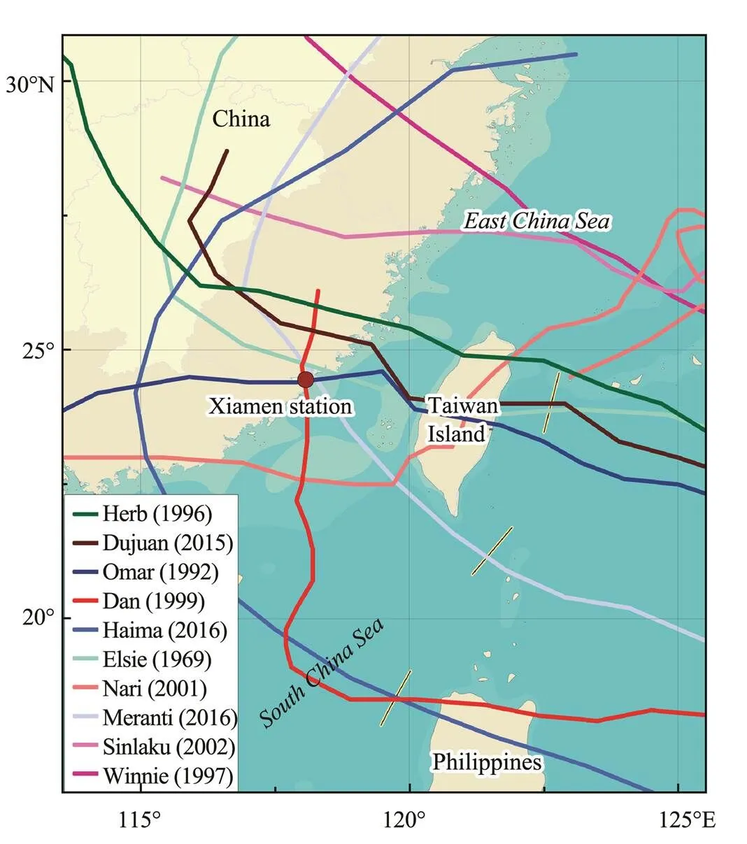
Fig.1 Location of Xiamen station and the tracking path of 10 typhoons. The track of typhoon Vongfong (2014) is be- yond the domain but its extreme water level is 730cm.
This dataset contains 60 years of tidal data from 1960–2019 with hourly observation intervals, good data quality, few interruptions, and integrity greater than 99.9%. Total potential error for tide data is estimated to be at 5cm (Peter, 2017). Astronomical tide and tidal constituent data were obtained from the T_TIDE package (Pawlowicz., 2002), the storm surge level data were obtained by subtracting the astronomical tides from the total water levels. The analysis of tidal observations yields the tidal amplitudes and phases at a set of discrete frequencies, which represent the different tidal constituents (Doodson, 1921, 1928). The M2stands for the lunar-based semi-diurnal tidal constituent, K1stands for the lunar-solar declination diurnal tidal constituent, andO1stands for the lunar declination diurnal tidal constituent.
The ratio of K1+O1constituent to M2constituent is 0.33, showing normal semi-diurnal characteristics, meaning that there are two high and low tides in each lunar day (24h and 50min), and the time interval between two adjacent high and low tides is approximately 12h and 25min. Harmonic analysis shows that the maximum astronomical tide, minimum astronomical tide, average maximum high water, average high water, and maximum astronomical tide surge (tide height relative to average water level) are 710, 29, 580, 569, and 350cm, respectively (Table 1).
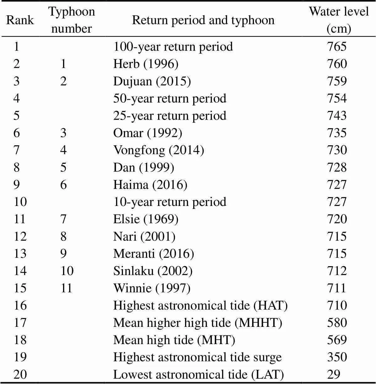
Table 1 Basic parameters of astronomical tides, extreme water levels and typical typhoons at Xiamen station,based on the zero-point water level in Xiamen
Fig.2 shows observed tidal and astronomical tide data through harmonic analysis. The root mean square error is 19cm, and the agreement index (AI)–an index that characterizes the degree of agreement between observation and simulated data–is 99.58%. Values close to 1 denote the good simulation effect and 99.58% of the agreement degree show that the astronomical and observation tides are perfectly matched. The root mean square error is approximately four times of the maximum error (5cm), meaning that the difference between the total water levels and as- tronomical tide levels is significant. The difference is the residual of the water level, which involves meteorological water level increase and sea level rise.
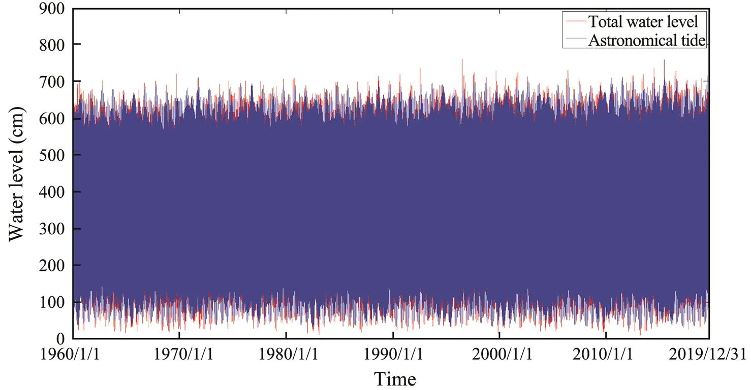
Fig.2 The time series of total water levels and astronomical tides from January 1, 1960 and to December 31, 2019.
2.2 Typhoon Probability
Xiamen experiences an average of 2.7 typhoons annually, and storm surges primarily occur from July to October, especially in August and September. Although tsunamis, extratropical cyclones, and cold waves can cause water level rise, this study only addresses water level rise caused by typhoons–the primary cause of extreme water level rise.
Typhoon Herb (1996) caused the highest water levels in the history of Xiamen, followed by typhoon Dujuan (2015). The storm surges caused by these two typhoons were much higher than those caused by other typhoons. Herb, the 8th typhoon in 1996, formed in the eastern Guam Island on July 23, 1996, became a typhoon in two days, gradually strengthened as it moved west-northwest, made landfall in Taiwan on July 31, and weakened to a tropical storm with a maximum wind speed of 45ms−1in the center. The tropical storm strengthened into a typhoon after crossing the Taiwan Strait and made landfall in the Fujian Province. Extremely high tides appeared along the coast of Fujian owing to the astronomical high tide and the funneling effect. Dujuan (2015), the 21st typhoon of 2015, formed in the northeastern Guam Ocean on September 21, 2015 and became a typhoon on September 25, with a ma- ximum wind speed of 55ms−1in the center. Dujuan made landfall in Taiwan on September 28, crossed into the Taiwan Strait the next day, and made landfall in Fujian. Omar (1992), Dan (1999), Meranti (2016), and other typhoons also caused the extreme rises in the sea levels as shown in Fig.1.
Vongfong (2014) did not affect Xiamen directly but caused a high water level of 732cm because of the combined influence of the typhoon periphery and cold air. Me- ranti (2016), the most devastating recent typhoon–made direct landfall in Xiamen with maximum winds of 52ms−1, and caused widespread damages. Eleven typhoons cau- sed the water levels higher than the highest astronomical tide as shown in Table 1. Of the 11 typhoons selected in this study, Vongfong (2014), Dan (1999), and Haima (2016) occurred in October, and eight occurred from July to Sep- tember. Xiamen experiences the astronomical spring tide in September and therefore even small water elevation changes can be disastrous. Fig.3 shows Xiamen station tidal data for five days during typhoons Omar (1992), Herb (1996), Dan (1999), Dujuan (2015), and Meranti (2016).
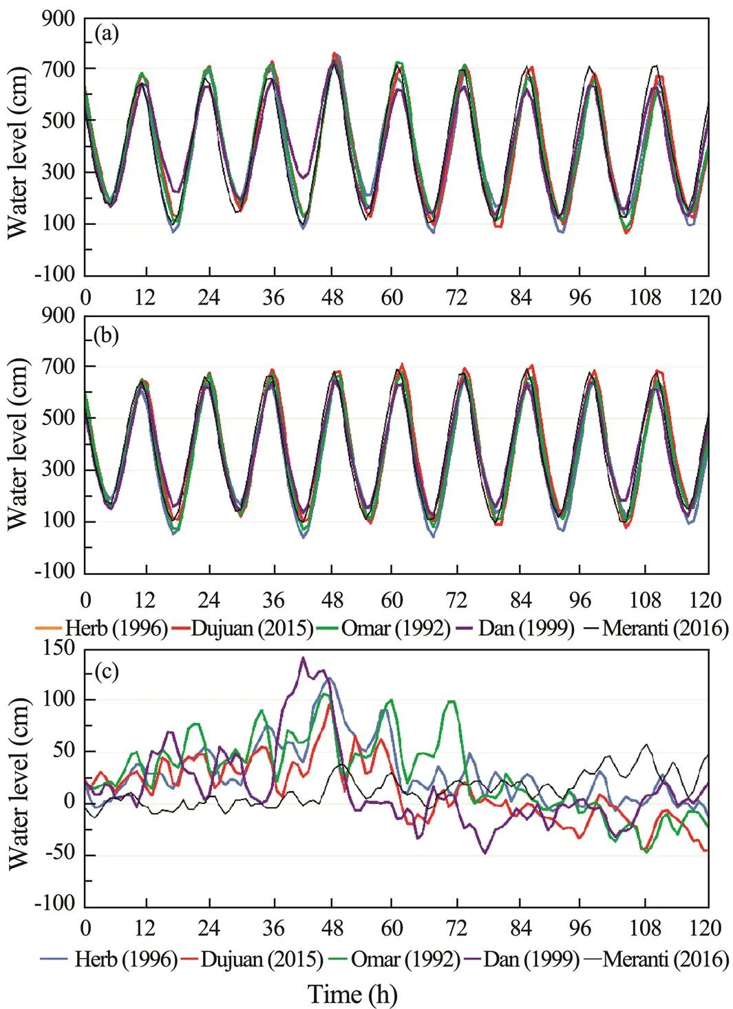
Fig.3 Five-day water level data for typhoons Herb (time zero is 01:00 July 30, 1996), Dujuan (time zero is 00:00 September 27, 2015), Omar (time zero is 01:00 August 28, 1992), Dan (time zero is 12:00 October 7, 1999), and Me- ranti (time zero is 01:00 September 16, 2016). (a), total water levels; (b), astronomical tides; (c), storm surges.
2.3 Interaction of Astronomical Tide and Storm Surge
Extreme tides are linked to storm surge, astronomical tide,and tide time. The overlap of storm surge and high tide caus- es extremely high tides. Xiamen station is in a semi-diurnal tidal sea, and the tidal period includes semi-diurnal (12.42h), daily (24.84h) and spring-neap periods (14.77d), and semi-annual (182.62d), annual (365.25d), and no- dal cycles (18.61yr).
Fig.4 shows the time intervals of each extreme water level relative to the highest astronomical tide. Nine out of 11 extreme water levels coincided with high tides; typhoons 2 and 3 arrived 1h before high tides. Typhoons 2 and 3 occurred 12h after maximum high tides, and typhoon 9 occurred 12h before the maximum high tide. Typhoons 6, 7, 8, and 10 coincided with the spring tide periods; other typhoons arrived within 2h before or after the spring tide periods, except typhoon 11, which occurred 3h before. Ty-phoon Haima arrived 6 days after the high-level time in semi-annual cycle and the remaining typhoons occurred before the onset of the cycle (1–2d in the case of typhoons 4 and 5).
Fig.5 shows the sea level increase at the time of highest tide and the proportion of astronomical tide. The average astronomical tide was 309cm, and the average proportion was 83.9%. Herb (1996) had the highest storm surge elevation of 115cm and the astronomical tide accounted for 71.2% of total water level elevation. Typhoon 11 Winnie (1997) had a water elevation of 87cm, in which the astronomical tide accounted for 75.2%. Typhoon 6 had the lowest water increase of 18cm and the astronomical tide accounted for 95.0%. The astronomical tide accounted for more than 90% of total water level during typhoons 6, 8 and 10. Assuming that typhoon Herb (1996) occurs during the highest astronomical tide, the highest water level will be 825cm, which is equivalent to a return period of more than 1000yr.
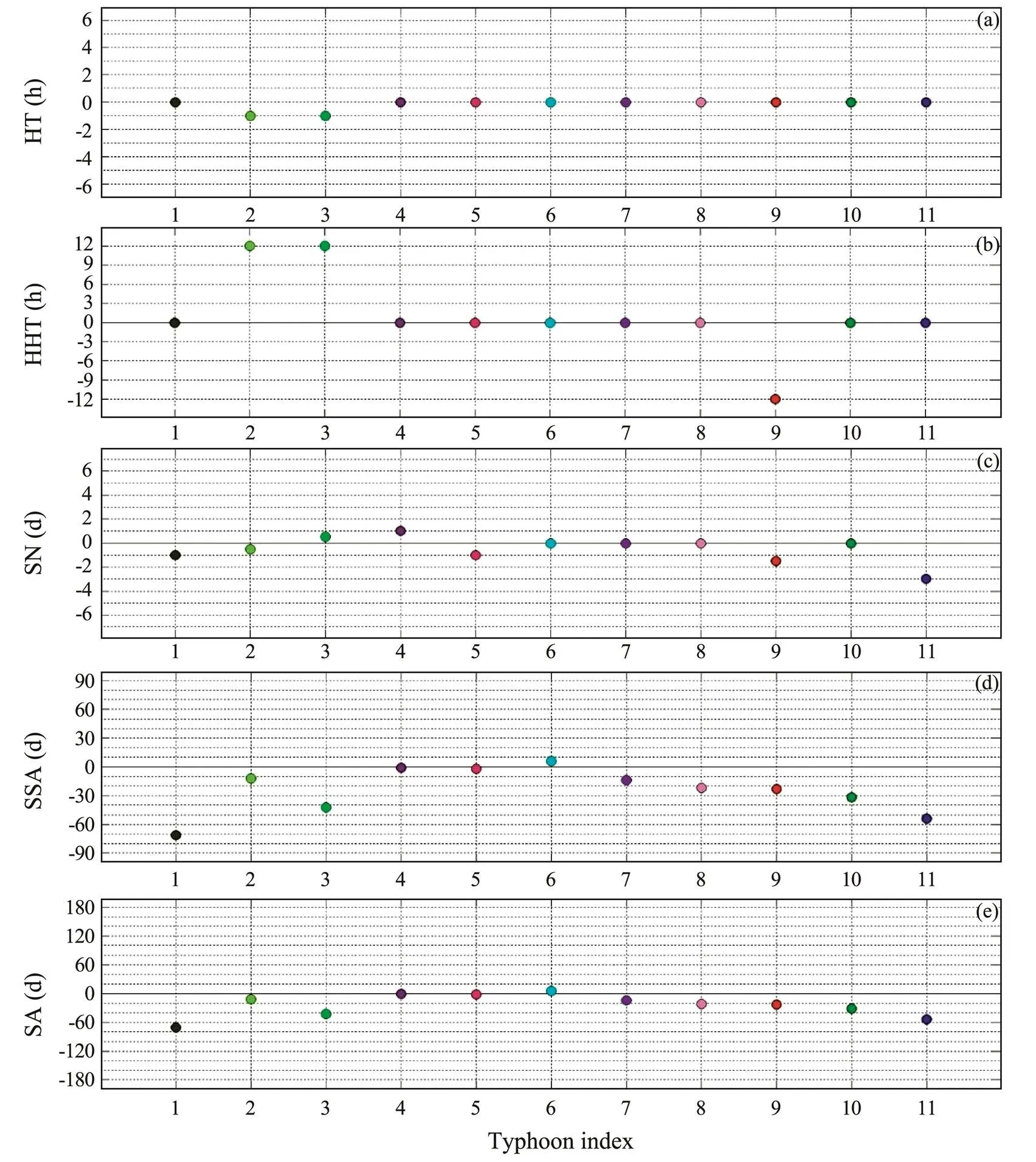
Fig.4 Extreme water level times of 11 typhoons related to the time of highest astronomical tides. Zero represents the time of the highest astronomical tides; negative and positive values indicate before and after astronomical tides, respectively. (a), high tide (HT); (b), higher high tide (HHT); (c), spring-neap tidal period (SN); (d), semi-annual cycle (SSA); (e), annual cycle (SA).

Fig.5 The height of maximum surges and astronomical ti- des, and the proportion of astronomical tide in actual sea levels during 11 typhoons. The astronomical tide is relative to the zero point of the tide.
3 Risk Assessment
3.1 Extreme Water Level Estimation
The Gumbel distribution is a common method for calculating the return period of marine meteorological and physical oceanographic elements and is often used to cal- culate high (low) water levels at different return periods (Wang and Jia, 1987; Hou, 1993; Qian., 2019). The Code of Hydrology for Sea Harbour (hereinafter referred to as the Code) of China stipulated that the Gumbel distribution should be used for water level frequency distribution curves. The Code suggests that other model curves, such as the lognormal, Weibull, and generalized extreme value (GEV) distributions can be selected according to the best fitting empirical accumulation frequency principle and the theoretical model. Three distribution curves inclu- ding Gumbel, Weibull and GEV methods are shown in Fig.6.The fit of the three distribution models is good when the re- turn period is less than 8yr. The Weibull distribution cur- ve gets worse with the increase of the return period. The GEV distribution curve fits not very well when the return period exceeds 20yr. The Gumbel distribution curve is the best fit to the observed water levels and is finally chosen for the estimation.
The probability distribution function of extreme water levels can be expressed as the following cumulative distribution function (Fisher and Tippett, 1928):

whereis the position parameter,is the scale parameter, andis the shape parameter.
The corresponding probability density function is:

The value ofdetermines the tail shape of the distribution;=0 denotes type-I extremum or Gumbel distributions.
Annual extreme water level data from 1960–2019 were sorted in descending order, and the Gumbel probability density distribution function was used to fit the 60-year extreme water level data as shown in Fig.7. Extreme water levels with the 10-yr, 25-yr, 50-yr, and 100-yr return periods were calculated and compared with observed extreme water levels and astronomical tides as shown in Table 1. Extreme water levels caused by Herb (1996) and Dujuan (2015) were much higher than those caused by other typhoons. The Gumbel distribution, which was calcu- lated without involving the data of typhoons, can be considered as the background to study the impact of these typhoons on Xiamen.
The 11 typhoons can be divided into three grades according to the extreme tides and water levels of the return periods. Herb (1996) and Dujuan (2015) were in the first grade with water levels of 760 and 759cm that correspond- ed to 76 and 71yr, respectively, according to the Gumbel curve. There were four second-grade typhoons with return periods from 10–25yr. The remaining five typhoons had return periods of fewer than 10yr. Meranti (2016), a third grade storm, caused serious damages in Xiamen with an ex- treme tidal level of 715cm.

Fig.6 Annual observed extreme water levels and different probability distribution curves to fit the water level variation during a return period.

Fig.7 The relative water levels and return periods of eleven storm surge events.
3.2 Sea Level Rise
The 60-yr tendency of sea level change was calculated by using the harmonic analysis results. Linear and quadra- tic nonlinear fittings were performed after anomaly changes to obtain linear and nonlinear sea level change tendencies, respectively.
The fitting formula are:


where Eq. (3) is the linear fitting formula, and Eq. (4) is the nonlinear fitting formula,is the month, andis sea level change (cm). According to the linear fitting formula, the sea level is rising at a rate of 0.306cm per year. The nonlinear fitting formula indicates the accelerating sea le- vel rise.
According to the fitting results, linear and nonlinear sea level rise in the next 10, 25, 50, and 100yr will be 3.06 and 3.33cm, 7.65 and 8.45cm, 15.30 and 17.30cm, 30.60 and 36.19cm, respectively. The nonlinear sea level rise of 36.19cm will be a very large value considering the highest astronomical tide elevation of 350cm.
The fifth IPCC report indicates that the rate of global sea level rise has been accelerating since the 20th century, by 1.7mmyr−1from 1901–2010 and 3.4mmyr−1from 1993–2016 (Wuebbles., 2017). Coastal sea levels in China rose by 3.2 and 3.8mmyr−1from 1980–2016 and 1993–2016, respectively. They are more than the average global sea level rise of 3.3mmyr−1 in the same period (Wang, 2018). In this work we estimate the linear and nonlinear sea level rise rates are of 3.1 and 3.3–3.6 mmyr−1, respectively. The values approximately agree withthose reported in previous researches (Han and Huang, 2008; Liu., 2010; Wang., 2011;Zuo., 2012).
Then, in 100yr, the highest sea levels involving the linear and nonlinear sea level rise factors are estimated to be 795.2 and 800.8cm, respectively, and correspond to a return period of approximately 1000yr according to the current Gumbel curve. Without the strong influence of typhoons Herb (1996) and Dujuan (2015), about 5.8–11.1cmwater level decrease will occur in the 10–100-yr return pe- riod (Fig.8).
3.3 Risk Assessment and Prediction
Hazard risk is the probability that a disastrous event occurs within a certain period. The formula for hazard risk in this paper is as following:

whereis the risk probability,is the probability of event occurrence, andis the number of years. The sea levels under the four situations with return periods of 10-, 25-, 50-, and 100-yr were converted into the correspondingvalues according to the Gumbel distribution curve, as shown in Fig.7.values are taken from 0 to 1000, and then the-value distribution curves can be obtained (Fig.9). The red, blue, dot, and black lines denote the four cases. The linear and nonlinear trends were applied to the estimation with and without Herb and Dujuan, respectively. The greater the number of assessed factors is and the higher the sea level is, the lower the risk probability for a given year is. For example, when the sea levels in a 10-yr return period without and with Herb and Dujuan are 721.9 and 734.7cm, the corresponding-values are 0.78 and 0.65, respectively. Thus, the probabilities of the sea level reaching 721.9 and 734.7cm within a 10-yr return period are 78% and 65%, respectively. This means that the hazard risk will increase if we exclude the influence of Herb and Dujuan in coastal engineering projects. The red line in Fig.9 represents the situation with Herb and Dujuan (also the situation for the Gumbel curve in Fig.7). The probabi- lity of this risk at the corresponding time of the return period is 63%–65%.
The differences between the curves and the horizontal axis and between the two curves are the total and relative risk degrees, respectively. The differences between the cur- ves gradually increase as the return period increases. With-out Herb and Dujuan, the risk probability will significantly increase, and the total risk degree will increase relatively with the increase of the return period. The risk probability for the 10-yr return period increases by a maximum of 13.4%, and the total risk degree within 10yr increases by 26.8%. The risk probability for the 25-yr return period increases by a maximum of 18.4%, and the total risk degrees within 10 and 25yr increase by 52.2% and 72.7%, respectively. The risk probability for the 50-yr return period increases by a maximum of 22.1%, and the total risk degrees within 10, 25, and 50yr increase by 74.0%, 62.0%, and 47.1%, respectively. The risk probability for the 100- yr return period increases by a maximum of 25.2%, and the total risk degrees in 10, 25, 50, and 100yr increase by 94.3%, 85.4%, 72.9%, and 54.4%, respectively.

Fig.8 The sea levels in 10-, 25-, 50-, and 100-yr return periods when typhoons and global sea level rise were involved.

Fig.9 Forecasted hazard risk curves when the return period is 10 (a), 25 (b), 50 (c), and 100 (d)yr.
The risk probability and total risk degrees are significantly reduced when the influence of sea level rise is considered. For return periods of less than 50yr, the risk pro- bability of predicted water levels according to the linear trend is reduced by a maximum of 5.4%–48.4%. The prediction based on the nonlinear trend for a 100-year return period decreases the risk probability by 56.9%. The total risk decreases by 3.1% for the 10-yr return period and by 75.4% and 69.7% within 10 and 100yr for the 100-yr period, respectively. For the nonlinear trend, the value increases 77.5% within 100yr.
4 Conclusions
In this study the extreme water levels are predicted and the risks are assessment at Xiamen station based on 60- year observation data. The interaction of astronomical tide and storm surge has been analyzed and the results show that typhoons Herb (1996) and Dujuan (2015) had the greatest impact on the distribution of extreme water levels. For the 100-yr return period, the total risk within 10, 25, 50, and 100yr increases by 94.3%, 85.4%, 72.9%, and54.4%, respectively. The simultaneous occurrence of Herb (1996) or Dujuan (2015) with the maximum astronomical tide would raise tidal levels by 800cm, which is exceed the 1000-year return period.
The average annual sea levels in Xiamen rose by 3.3–3.6mmyr−1from 1960–2019 and the rate of sea level rise is still increasing. Relative sea level rise in the next 10, 25, 50, and 100yr are predicted to be 3.33, 8.45, 17.3, and 36.19cm respectively. For a return period of fewer than 50yr, the predictions when the linear sea level rise is considered get a lower risk probability, whereas the nonlinear trend is much more important for the 100-yr return period. The risk probability and risk degree are reduced maxi- mally by 56.9% and 77.5%, respectively, over 100yr when non-linear trend is applied.
Acknowledgements
This study is supported by the National Key Research and Development Program of China (No. 2016YFC140 1103), the NSFC-Shandong Joint Foundation (No. U1706 226), the National Natural Science Foundation of China (No.51779236), and the Open Fund of Shandong Province Key Laboratory of Ocean Engineering (No. kloe201903).
Dong, J. X., Zhang, T. Y., and Fu, X., 2008. Calculation of the storm surges in the Shacheng Bay in Fujian Province in 100 years return periods., 27: 9-16.
Doodson, A.T., 1921. The harmonic development of the tide-ge- nerating potential.,100: 305-329.
Doodson, A.T., 1928. The analysis of tidal observations., 227: 223-279.
Fan, L. L., and Wang, Y. Y., 2017. Parameter estimation and case analysis of based on generalized extreme value distri- bution., 38 (3):13-17 (in Chinese with English abstract).
Fisher, R. A., and Tippett, L. H. C., 1928. Limittimg forms of the frequency distribution of the largest or smaHest member of a sample., 24: 180-190.
Han, G., and Huang, W., 2008. Pacific decadal oscillation and sea level variability in the Bohai, Yellow, and East China Seas., 38: 2772-2783.
Hou, R. K., 1993. Calculating the annual maximum water level using the Gumbel extreme value distribution., 3: 126-129.
Huang, W. R., Xu, S. D., and Nnaji, S., 2008. Evaluation of GEVmodel for frequency analysis of annual maximum water levels in the coast of United States., 35 (11-12): 1132-1147.
Jiang, Y. W., Wu, P. M., and Xu, J. D., 2000. A model with inter- action of tide and surge for Xiamen Harbor., 22: 1-6.
Liu, X., Liu, Y., Guo, L., Rong, Z. R., Gu, Y. Z., and Liu, Y. H., 2010. Interannual changes of sea level in the two regions of East China Sea and different responses to ENSO., 72: 215-226.
Pawlowicz, R., Beardsley, B., and Lentz, S., 2002. Classical tidalharmonic analysis including error estimates in MATLAB using T-TIDE., 28(8): 929-937.
Peter, B., 2017. Tide-surge historical assessment of extreme water levels for the St. Johns River: 1928–2017.,553: 624-636.
Pirazzoli, P. A., and Tomasin, A., 2007. Estimation of return pe- riods for extreme sea levels: A simplified empirical correction of the joint probabilities method with examples from the French Atlantic coast and three ports in the southwest of the UK., 57(2): 91-107.
Qian, L. X., Wang, H. R., Zhang, R., and Jiao, Z. Q., 2019. Gum- bel extreme hydrological frequency analysis model in situa- tions of insufficient data., 51 (5): 41-48 (in Chinese with English abstract).
Samuels, P. G., and Burt, N., 2002. A new joint probability ap- praisal of flood risk, proceedings of the institution of civil en- gineers.–, 154(2): 109-115.
Shi, X. W., Tan, J., Guo, Z. X., and Liu, Q. Z., 2013. A review of risk assessment of storm surge disaster., 28 (8): 866-874 (in Chinese with English abstract).
Sobey, R. J., 2005. Extreme low and high water levels., 52(1): 63-77.
Toro, G. R., Resio, D. T., Divoky, D., Niedoroda, A.W., and Reed, C., 2010. Efficient joint-probability methods for hurri- cane surge frequency analysis., 37: 125-134.
Vogel, R. M., Tomas, W. J., and Mcmahon, T. A., 1993. Flood-flow frequency model selection in southwestern United States., 119: 353-366.
Walton, T. L. J., 2000. Distributions for storm surge extremes., 27: 1279-1293.
Wang, H., Fan, W. J., Zhang, J. L., and Mu, L., 2011. The cha- racteristics of sea level changes along the coast of China in recent 31 years., 30 (6): 637-643 (in Chinese with English abstract).
Wang, H., Liu, K. X., Fan, W. J.,Feng, J. L., Wang, G. S., Zhang, J. L.,., 2018. Aanalysis on the sealevel anomaly high of 2016 in China coastal area., 40 (2): 43-52 (in Chinese with English abstract).
Wang, J., and Jia, S. D., 1987. A program for extreme value ana- lysis by using the Gumbel method., 6: 87-91.
Wang, Y. J., Zhang, R., Qian, L. X., Ge, S. S., and Wang, F., 2016.Model for probabilistic risk assessment in extreme high water level caused by rising sea level and its application–A case study in Ningbo., 31 (1): 213-218 (in Chinese with English abstract).
Wuebbles, D. J., Fahey, D. W., Hibbard, K. A., Dokken, D. J.,Stewart, B. C., and Maycock, T. K., 2017.. Marine Research Press, Washington, D. C., 470pp.
Yuan, F. C., Wu, X. R., and Lu, J. F., 2018. Statistical characte- ristics of storm surges in central and southern Fujian coast., 35:68-75 (in Chinese with English abstract).
Zhang, H., and Sheng, J., 2015. Examination of extreme sea le- vels due to storm surges and tides over the Northwest Pacific Ocean., 93: 81-97.
Zhu, Y. M., and Li, Z. L., 2011. Sea level variation and the effectto water level extreme distribution estimate in South China.,4:126-133 (in Chinese with English abstract).
Zuo, J., He, Q., and Chen, C., 2012. Sea level variability in East China Sea and its response to ENSO., 5: 164-174.
November 19, 2020;
February 22, 2021;
July 31, 2021
© Ocean University of China, Science Press and Springer-Verlag GmbH Germany 2022
. E-mail: wzf1984@ouc.edu.cn
(Edited by Chen Wenwen)
杂志排行
Journal of Ocean University of China的其它文章
- Study of the Wind Conditions in the South China Sea and Its Adjacent Sea Area
- A Spatiotemporal Interactive Processing Bias Correction Method for Operational Ocean Wave Forecasts
- Underwater Target Detection Based on Reinforcement Learning and Ant Colony Optimization
- Polar Sea Ice Identification and Classification Based on HY-2A/SCAT Data
- Thermo-Rheological Structure and Passive Continental Margin Rifting in the Qiongdongnan Basin,South China Sea, China
- Effect of Penetration Rates on the Piezocone Penetration Test in the Yellow River Delta Silt
