Study of the Wind Conditions in the South China Sea and Its Adjacent Sea Area

YAN Zhiduo, WANG Zhenlu, and PANG Liang

Study of the Wind Conditions in the South China Sea and Its Adjacent Sea Area

YAN Zhiduo1), #, WANG Zhenlu1), 2), #, and PANG Liang1), 2), *

1) College of Engineering, Ocean University of China, Qingdao 266100, China 2) Shandong Province Key Laboratory of Ocean Engineering, Ocean University of China, Qingdao 266100, China

An increasing number of marine structures have been built for coastal protection and marine development in recent years, and wind, which is crucial to marine structures, should be analyzed. Therefore, typhoon frequency, wind climate, wind energy assessment, and extreme wind speed in the South China Sea (SCS) are investigated in detail in this study. The data are obtained from the China Meteorological Administration, the European Centre for Medium-range Weather Forecasts, and the National Centers for Environmental Prediction. The offshore wind energy potential is analyzed at five sites near the coast. The spatial and monthly frequencies of tropical cyclones for different intensity categories are analyzed. The extreme wind speed is fitted by five distribution models, and the generalized extreme value (GEV) distribution is selected as the most suitable function according to the goodness of fit. The spatial distributions of extreme wind speeds in the SCS are plotted on the basis of the GEV distribution and ERA5 data sets. The influences of the distribution models and data sets on the calculated results are discussed. Moreover, the monthly extreme wind speed and comparison with the results of previous studies are analyzed. This study provides a reference for the design of wind turbines.

tropical cyclone; South China Sea; extreme wind speed; GEV distribution; wind energy assessment

1 Introduction

Abundant resources, such as petroleum and combustible ice, are stored in the South China Sea (SCS). Moreover, the maritime industry, which involves production, shipping, and transportation, requires suitable wind conditions. The SCS is located in the monsoon zone, where typhoons are one of the most frequent activities. Economic losses and even casualties in coastal cities near the SCS are often unavoidable when typhoons hit. Typhoons cause disasters in coastal cities but contain tremendous energy. The exploitation and utilization of marine renewable energy, such as offshore wind energy and wave energy, are increasingly considered by ocean planners and engineers. Therefore, the analysis of wind conditions can help people make better decisions in the process of energy exploitation, including design, construction, and operation. More- over, extreme wind speed analysis can minimize coastal hazards and economic losses.

Zheng and Pan(2014) and Yang(2017) analyzed the wind power industry in China and reported that offshore wind power has considerable potential. Wang(2018) determined that offshore wind energy is stronger than nearshore or inland wind energy as evaluated on the basis of 30-year data from the SCS. Wind energy resource assessment in the China Sea guides the location of wind and wave power plants (Zheng, 2012, 2013). Wind power potential and variability in different sea areas have been assessed by several scholars (Geyer, 2015; Ali, 2018; Chidean, 2018). Moreover, several researchers have made significant contributions to the assessment models (Hasager, 2015; Kantar, 2018) and driving wind fields for the wave models (Shao, 2018).

However, the SCS, which is located in the monsoon zone, is one of the sea areas most severely affected by typhoons. Moreover, the waves and storm surges induced by typhoons can destroy marine structures and cause disasters in coastal regions (Wu, 2014, 2018). Therefore, extreme wind speeds must be considered in marine structure design and coastal protection, and the accurate estimation of extreme wind speeds for wind turbine design is important. The exact calculation of extreme wind speed is critical to the safety of structures and the reduction of economic losses. The design standard adopts wind speed with a return period calculated by fitting the samples to the corresponding distributions. The Weibull, Gumbel, and generalized extreme value (GEV) distributions are widely used for extreme wind speed estimation (Weisser, 2003; Lombardo, 2009; Lee, 2012; Ohunakin and Akinnawonu, 2012; Yao, 2012; Nedaei, 2014; Tizpar, 2014; Wang, 2015). Moreover, several other models that can estimate extreme wind speeds,, peak-over-threshold (Gao, 2018; Liang, 2019), multivariate compound extreme value distribution (Liu, 2006; Pang, 2007; Liu, 2010), environmental contour line (Haver, 2009), and deductive methods (Yan, 2020a, 2020c), have been continuously assessed and improved.

The wind conditions vary for different months at a given location, which makes wind climate analysis valuable. Zheng(2018) analyzed the wind climate, including regular and extreme wind speeds. Zheng(2020) analyzed the extreme wind speed distribution in the China Sea in each season. Chen(2020) established the monthly frequency indices of typhoons during active seasons. Moreover, sea surface temperature and precipitation rate vary once a typhoon occurs (Haghroosta, 2017). Niroomandi(2018) reported that return levels with a 100-year return period calculated from the GEV and generalized Pareto (GP) distributions of the annual maximum data were higher than those of the monthly maximum data by 10%. Young and Donelan (2018) analyzed three extensive global wind speed data sets to investigate the global wind speed climate. Campos and Soares (2018) investigated the spatial characteristics of wind speed statistics in the oceanic areas of Portugal. Yan(2020b) analyzed extreme wind speed estimates on the basis of different distribution models. Cannon(2015) estimated the frequency of relatively short-lived extreme events using reanalysis data. Wang and Zhao (2019) analyzed the wind characteristics in the Nansha Area.

Previous studies mainly improved the methods but did not conduct analyses of the overall spatial distribution. Site selection for ocean engineering and the development and transportation of marine resources all need to have a holistic grasp on the spatial distribution of the marine environment. A full understanding of spatial wind distribution can reduce costs and disasters. In this study, wind conditions in the SCS, including seasonal characteristics, wind energy assessment, long-term extreme value analysis, and spatial wind speed analysis, are analyzed. This paper is organized as follows: In Section 2, an overview of the research region and data is provided; in Section 3, we analyzed regular wind in the SCS; in Section 4, we investigated extreme wind speeds in the SCS; in Section 5, contrastive analysis of extreme wind speed estimation is discussed; in Section 6, the conclusions are provided.

2 Data and Methodology

2.1 Research Area

The study area is located at longitude 100˚ to 125˚E and latitude 0˚ to 30˚N (Fig.1). The SCS is a marginal sea or an arm of the western Pacific Ocean, south of the Chinese mainland and north of the equator. The area of the SCS is approximately 3500000km2, of which China’s territorial sea area is approximately 2100000km2. The mean water depth is approximately 1212m, and the maximum depth is 5559m.

Tropical cyclones (TCs) in the SCS are categorized into two types,, one is from the Western Pacific Ocean and the other is generated in the SCS. TCs occur, develop, and pass through only under suitable conditions. Geographically, tropical depressions occur in the SCS as far south as 5.5˚N, as far west as 107.5˚E, and as far north as 24˚N. Since April, the location of the TC origin gradually moves to the north and concentrates at 15˚ to 20˚E and 110˚ to 120˚N from July to September. Since June, the location of the TC origin gradually moves to the northeast and reaches its northernmost and easternmost positions in September. After September, the location of the TC origin moves to the southwest, but the concentration phenomenon becomes less obvious. Tropical storms, which can intensify into typhoons, are geographically located in water depths of more than 150m. The contours of the 150m water depths of the SCS are north-northeast to south-southwest, which are similar to the central axis of a tropical storm that intensifies into a typhoon. The movements and other changes in the concentration areas of typhoons in the SCS are related to the ebb and flow of the east wind and southwest monsoon, as well as the invasion of strong cold air.

Fig.1 Profile of the research area and locations of the calculated points.

2.2 Method and Model Introduction

To facilitate the use of engineering and design, the collected wind data are often statistically sorted and drawn into a wind chart, which is also known as a wind rose chart because it looks like a blooming rose. In this study, regular wind in the SCS is analyzed using the wind rose chart divided into 36 directions, mainly representing the distribution of wind speed and direction and occurrence frequency in a certain place.

The extreme wind speed with a certain return period is often used to determine the design of wind speeds in ocean engineering. The design standard of marine environmental elements is based on the long-term observation data of environmental elements and the results of statistical analysis. An appropriate extreme value estimation method and a specific recurrence period are selected according to the needs of the project, and the extreme value for this recurrence period is considered the engineering design standard.

According to the extreme value theory, extreme wind speed can be estimated using the extreme value distribution. However, the estimated results will be different whenusing different distribution models. In this study, five distributionmodelswillbeusedtoestimateextremewindspeed. The five distribution models are expressed as follows:

1) Weibull distribution with two parameters (Weibull- 2par):

2) Weibull distribution with three parameters (Weibull- 3par)

3) GEV distribution

4) Log-normal distribution

5) GP distribution

2.3 Data Introduction

The data utilized in this study are obtained from the best track data set of China Meteorological Administration Shanghai Typhoon Institute (CMA-STI) and the ERA5 data sets of the European Centre for Medium-range Weather Forecasts (ECMWF). The best track data set of CMA-STI records the typhoon information, including the year of occurrence, typhoon number, typhoon name, time, longitude and latitude of the typhoon center, and central pressure in the Northwestern Pacific Ocean. The growth process of a tropical depression into a typhoon and the weakening of a typhoon into a tropical depression are recorded in the data set (Ying, 2014). The recording frequency is four observations per day. The data period used in this study is from 1979 to 2018, with a total of 1208 TCs oc-curring during these four decades. Fig.2 shows the TC tracks through the research area from 1979 to 2018, with the colors denoting different TC tracks.

The data set from the ECMWF covers the period from 1950 to the present with intervals of 1h. The data set utilized in this study covers the period from 1979 to 2018. The wind field is obtained from a height of 10m and consists of two wind components, namely,and. The spatial resolution is 0.25˚. Moreover, the data obtained from the National Centers for Environmental Prediction (NCEP) Climate Forecast System Reanalysis from 1979 to 2010 were compared with the ERA5 data sets.

Five typical points (, A, B, C, D, and E) near the coast are selected to analyze the wind energy potential. The positions of these points are shown as green points in Fig.1. Moreover, four calculated points (, P1, P2, P3, and P4) are selected to analyze the extreme wind speed and wind climate, which are shown as red points in Fig.1. The four points represent the four directions in the SCS. The longitude and latitude of the calculated points are shown in Table 1.

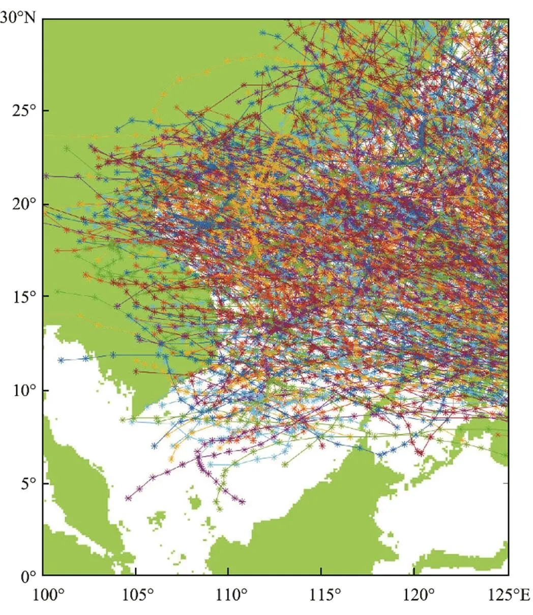
Fig.2 Typhoon tracks through the research area from 1979 to 2018.

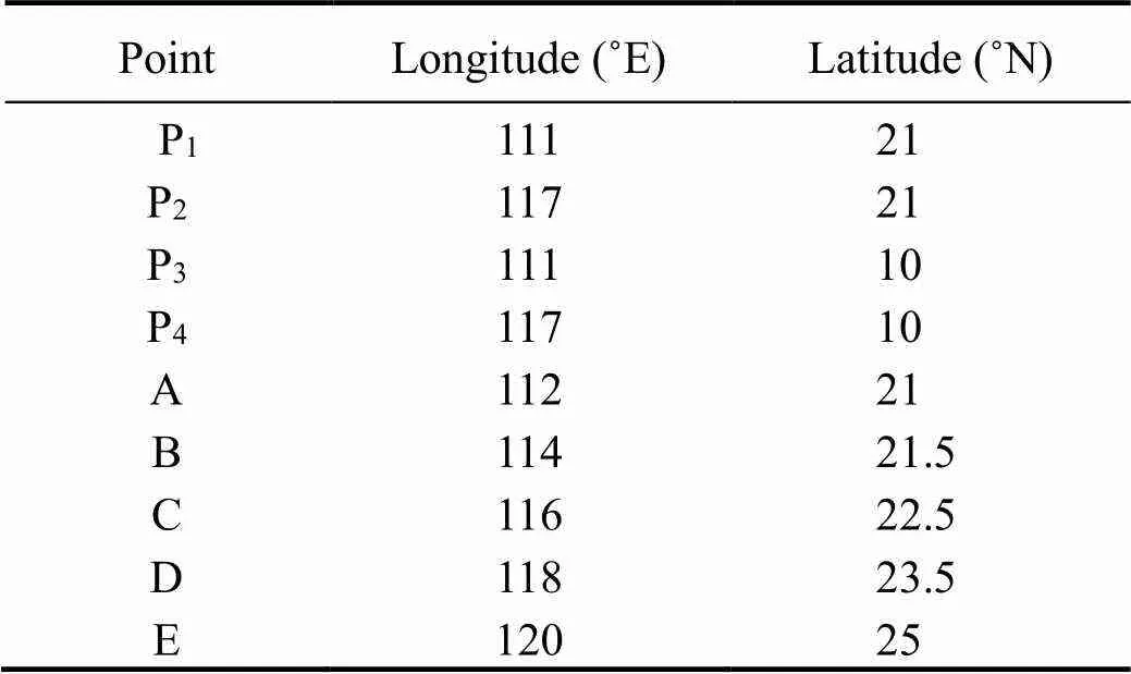
Table 1 Longitude and latitude of the calculated points

3 Regular Wind Analysis

3.1 Wind Speed and Direction

Regular wind can influence the power generation efficiency of wind turbines. The wind speed distribution and wind direction are critical factors that need to be considered in the design of wind turbines. The averaged wind fields in each month according to the ERA5 data sets are shown in Fig.3. As shown in the figure, the wind speed at sea is significantly higher than that on land. In January,the wind direction was mainly southwest, but that near the Bashi Channel was west. In February, wind in the northern part of the SCS and Bashi Strait changed to a westerly direction, whereas wind in the other parts was mainly in the southwest direction. In March, wind in most parts of the SCS shifted to the west, whereas wind in the other parts was similar to that in February. In April, wind in the southwest part of the Hainan Island shifted to the northwest, whereas wind in the other parts remained unchanged. In May, the wind speed on the west side of the Indochina Peninsula was relatively high, and the wind direction shifted to the north. In June, the wind speed in the south of the SCS was relatively high, and the wind direction was north- east, whereas the wind direction in the north of the SCS was north. July was similar to June. In August, the wind speed in the north of the SCS decreased. In September, the wind speed in the central and northern parts of the SCS was relatively low, whereas the wind speed in the Taiwan Strait was relatively high, and the wind direction was southwest. In October, the wind speed in the north of the SCS increased, and the wind direction was mainly southwest. In November, the wind speed in the entire SCS and the East China Sea was the same, and the wind direction was southwest. Compared with that in November, the wind speed in the southern part of the SCS in December increased slightly.

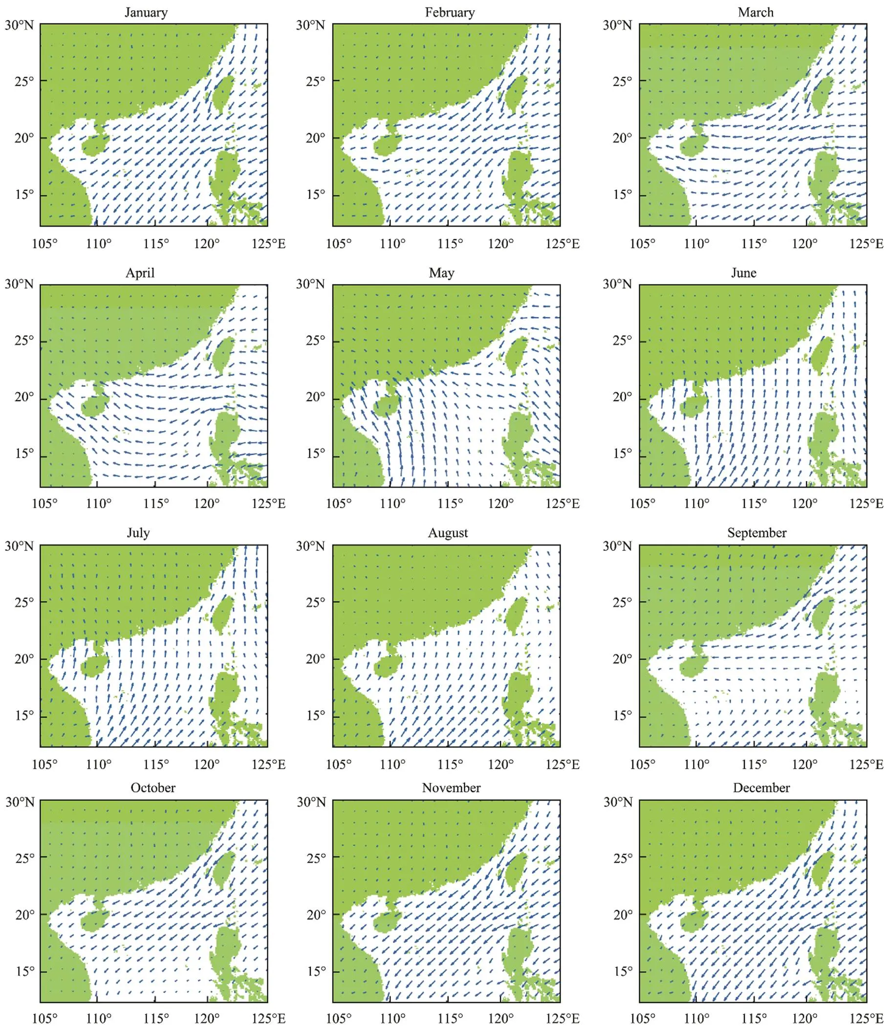
Fig.3 Average wind fields in each month based on the ERA5 data sets in the South China Sea (SCS).

The above-average wind field was utilized to analyze the distribution of wind speed and direction in space but not in frequency. To analyze the occurrence frequency of different winds, four representative points were selected in this study to draw a wind rose chart (Fig.4) on the basis of the ERA5 data sets. The longitude and latitude coordinates of the four points (, P1, P2, P3, and P4) are shown in Table 1, and their locations are shown in Fig.1. As shown in Fig.4, P1is located north of the SCS, near Guangdong Province. The wind direction is mainly distributed in the west, northwest, and west-southwest, and the wind speed is approximately 5–10ms−1. P2is located northeast of the SCS. The wind direction is mainly south- west, which is relatively fixed throughout the year, and the wind speed is approximately 5–15ms−1. P3is located southwest of the SCS. The wind direction is mainly south- west and northeast, and the wind speed is approximately 15ms−1. P4is located southeast of the SCS, and the wind direction is mainly southwest, followed by northeast. The wind speed is approximately 5–10ms−1, sometimes reaching more than 10ms−1.

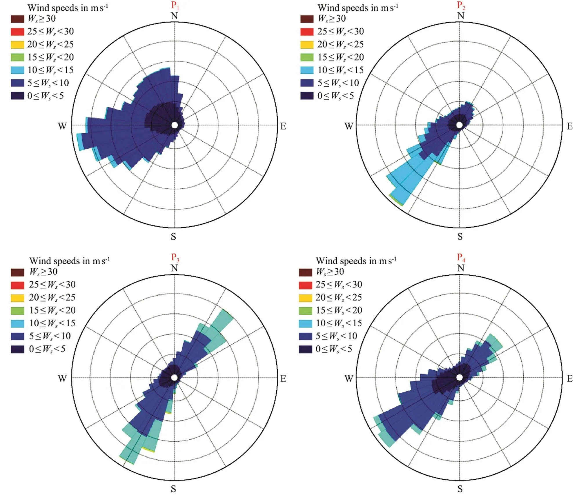
Fig.4 Wind rose diagrams of the SCS.

3.2 Wind Energy Assessment

Offshore wind energy assessments are important for the selection of wind farm positions. Five points near the coast (green points in Fig.1) are selected to analyze the wind energy potential in terms of two factors (, availability and capacity factors). The availability factor (A) indicates the probability of wind turbine operation. This factor can be expressed as follows:

The capacity factor (C) reflects the wind turbine productivity. This factor can be expressed as follows:

In Eqs. (6) and (7),v,v, andvdenote the cut-in, rated, and cut-out speeds, and their values are 3, 12.5, and 25 ms−1, respectively, in this study.() denotes the probability density function (PDF) of wind speed, and() denotes the cumulative distribution function (CDF) of wind speed. By analyzing the frequency histogram of wind speed from 1979 to 2018, we find it difficult to determine a suitable fitting function for all five points. Moreover, errors exist in the fitting distribution. Therefore, the empirical distribution is used to fit the wind speed in the subsequent calculations. The PDF and CDF are numerical; these parameters are calculated from the sample and do not require any assumptions regarding the form of the distribution. The PDF of wind speed is shown in Fig.5. TheAandCvalues at the five sites are shown in Table 2. According to the table, from point A to E, the values ofAare similar, and the values ofCincrease. This finding indicates that the wind turbine productivity offshore of the SCS increases from southwest to northeast. Moreover, the values ofAindicate that the wind speeds are within the power generation range of more than 88% of the time.

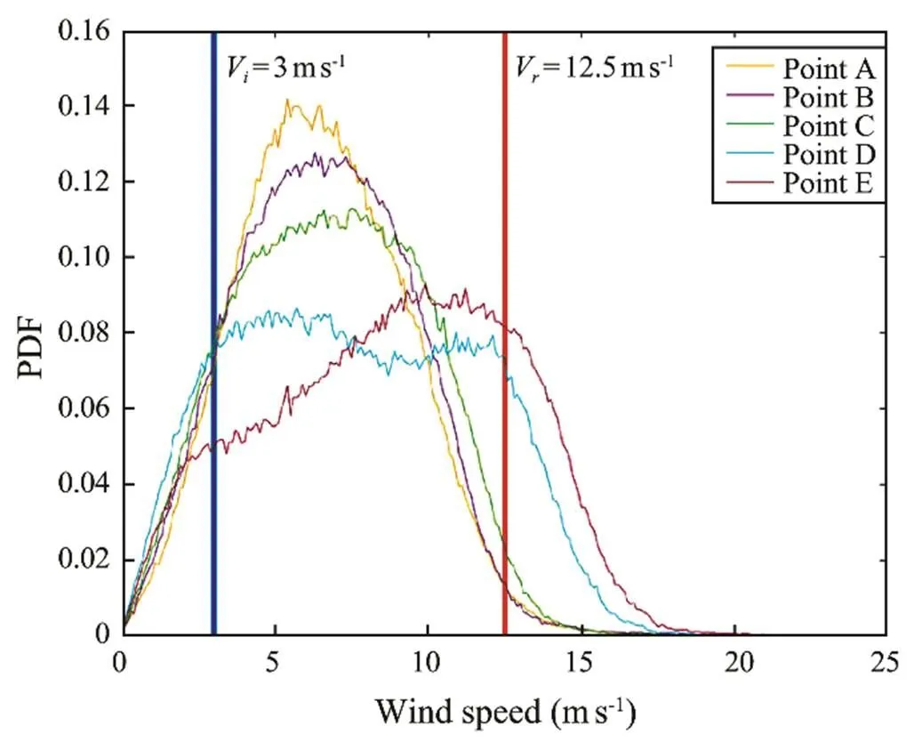
Fig.5 Distribution of wind speed in five coastal sites.

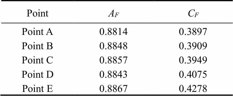
Table 2 AF and CF values of five coastal sites

4 Extreme Wind Speed Analysis

4.1 Frequency Analysis of TC

A total of 1208 TCs occurred in the Northwest Pacific (NWP) from 1979 to 2018, of which 688 passed through the research area of this study. The frequency of TCs oc-curring in the NWP and passing through the research area in each year is shown in Fig.6. The figure shows that TCs generally occur approximately 30 times annually on average in the NWP, of which the maximum was 40 times in 1989 and 1994 and the minimum was 18 times in 2010. The maximum frequency of TCs occurring in the SCS was 24 in 1980, and the minimum frequency of TCs occurring in the SCS was 10 in 1997. The comparison between the number of TCs occurring in NWP and SCS shows that more than half of the TCs occurring in NWP passed through the SCS.

The monthly frequency statistics of TCs occurring from 1979 to 2018 are shown in Fig.7. Notably, the trend of frequency in each month is the same in both NWP and SCS. Moreover, more TCs occur in summer and autumn and fewer TCs occur in spring and winter. The three months with the largest number of TCs are July, August, and September, more than half of the entire year in both NWP and SCS. In these three months, more than two TCs passed through the SCS in each month on average. Moreover, the number of TCs that passed through the SCS accounts for a large proportion of TCs occurring in NWP in November and December. This finding can be attributed to the fact that positive relative vorticity and weak vertical wind shear are more easily generated in winter in the SCS, which favor TC genesis in this region (Shi, 2020).

The category intensity of TCs is classified from least intense to most intense. The monthly frequency statistics of different-intensity TCs passing through the research area from 1979 to 2018 are shown in Fig.8. Notably, tropical storms are the most frequent of the six types of TCs, particularly in July and August. The other types of TCs occur with similar frequency. From June to November, the other types of TCs occur every two months. Super typhoons generally occur from July to October.

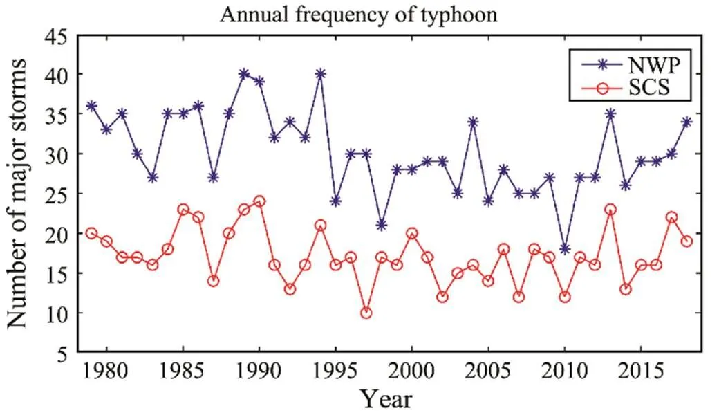
Fig.6 Number of typhoons occurring in the NWP and SCS from 1979 to 2018.

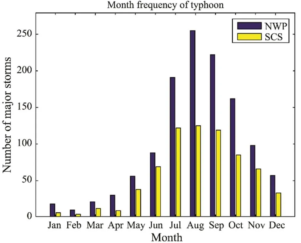
Fig.7 Monthly distribution of the frequency of TCs from 1979 to 2018.

The spatial frequency statistics of different-intensity TCs from 1979 to 2018 are shown in Fig.9. Frequency represents the number of TCs passing through a 1˚×1˚ grid from 1979 to 2018. TCs with a strong intensity occur at a low frequency. From tropical depressions to typhoons, those with a strong intensity are more likely to occur near the coast, with a high frequency in the north of the SCS and east of the Hainan Island. Severe typhoons and super typhoons rarely occur in the SCS but frequently occur in the east of the Bashi Channel and the Philippines.

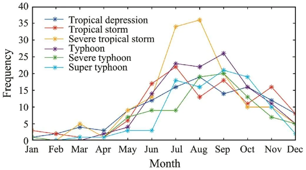
Fig.8 Monthly frequency statistics of different-intensity TCs passing through the research area from 1979 to 2018.

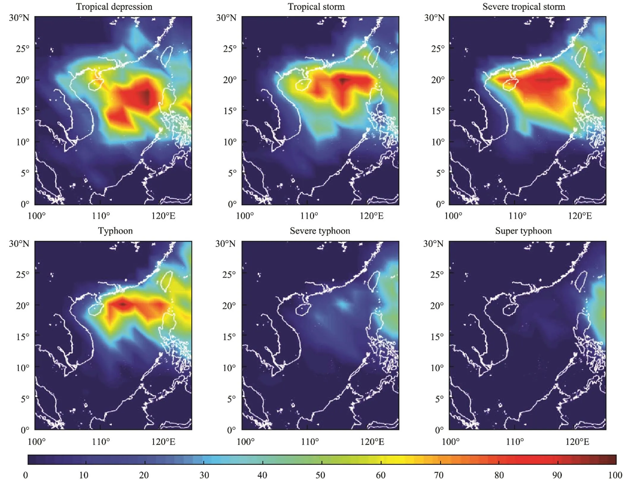
Fig.9 Spatial frequency statistics of different-intensity TCs passing through the research area from 1979 to 2018.

4.2 Extreme Value Analysis of Wind Speed

The estimation of extreme wind speed is critical to the safety of marine structures, such as offshore wind turbines. The design standard of wind speed is expressed as the maximum speed with a return period. In general, the extreme wind speed is estimated by fitting the samples to the corresponding probability distributions, and the wind speed of a certain return period is calculated on the basis of the probability distribution. In this study, five probability distributions (, GP, GEV, Weibull-3par, Weibull-2par, and log-normal) are selected to analyze the extreme wind speed in the SCS. The sample of the GP distribution is the threshold sample, and the sample of the other distributions is the annual maximum value sample. The fitted distribution function and Q-Q plot of all five distribution models at the four sites (P1–P4shown in Fig.1), which intuitively reflect the goodness of fit, are shown in Fig.10. In the left subplots, the closer the distribution function curve to the empirical distribution curve is, the better the fitting effect. In the right subplots, the closer the point to the red line is, the better the fitting effect. To determine the most suitable distribution to estimate the extreme wind speed, the Kolmogorov-Smirnov (KS) test is applied to the fitting distribution. Thevalue of the KS test can reflect the goodness of fit quantitatively, as shown in Table 3. A greatervalue reflects a better fit. According to the table, for thevalues of the four sites, the GEV distribution has the largest mean value and the lowest standard deviation (Std). Therefore, the GEV distribution is used to calculate the extreme wind speed in the spatial distribution of the SCS.

Fig.10 Distribution function curve and Q-Q plot fitted by five distribution models at four sites.

On the basis of the GEV distribution, the design wind speeds with 50-year and 100-year return periods for the research area are shown in Fig.11. Extreme wind speed values with 50-year and 100-year return periods have the same distribution characteristics. As shown in the figure, the highest value of extreme wind speed can be observed near latitude 15˚N. Moreover, the extreme value of the west is greater than that of the east because the TC strengthens from the east to the west in this region. The highest values of the 50-year and 100-year return periods are higher than 40 and 50ms−1, respectively. In the north, including the coastal area, the extreme value decreases slightly, but the value of the 100-year return period is still higher than 30ms−1. The southern area has the smallest values because the TC does not develop sufficiently or TC is rerely happened.

Table 3 p values of the Kolmogorov-Smirnov tests for different distribution models and points

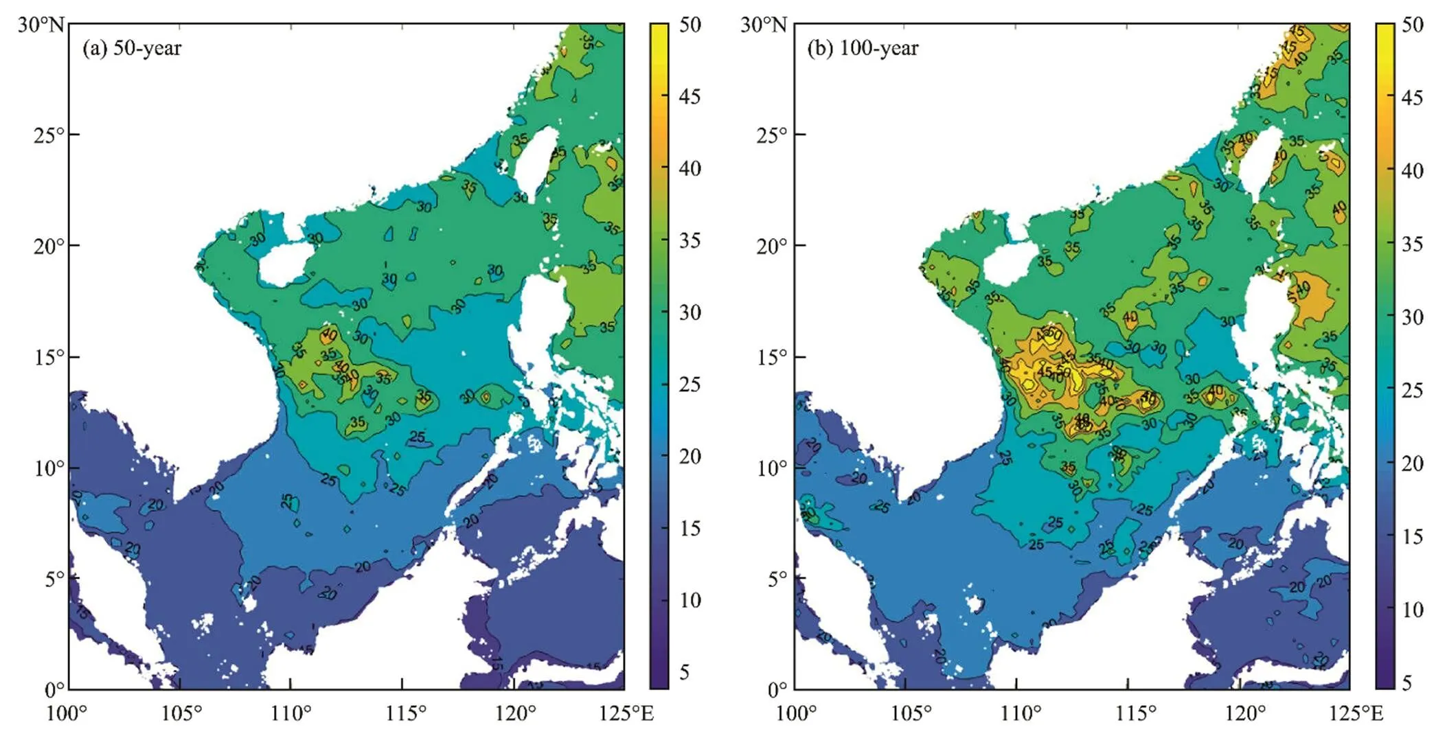
Fig.11 Extreme wind speeds with 50-year (a) and 100-year (b) return periods in the SCS.

5 Discussion

5.1 Results Influenced by the Distribution Model

The tail shape of each distribution is different; as a result, the predicted extreme wind speed is also different. To determine the difference in extreme wind speed estimated using different distribution models, the return level of the corresponding return period is calculated, as shown in Fig.12 and Table 4. The results indicate that the values calculated using the GEV distribution are higher than those calculated using the other distributions, except for the GP distribution, particularly for a long return period.

Moreover, the standard error (SE) is calculated to evaluate the differences between different methods. The SE can be expressed as follows:

where xi denotes the results calculated using the other methods and x′ denotes the results calculated using the GEV distribution. The SE values listed in Table 4 indicate that the return levels of 10, 50, and 100 years have small differences, whereas the return levels of 1000 years have large differences. Moreover, Fig.12 shows that, when the exceedance probability is less than 10−2 (i.e., the return period is longer than 100 years), the GEV distribution diverges. Therefore, we recommend the use of the GEV distribution to calculate the extreme wind speed when the return period is shorter than 100 years. Moreover, other methods should be used when the return period is longer than 100 years.

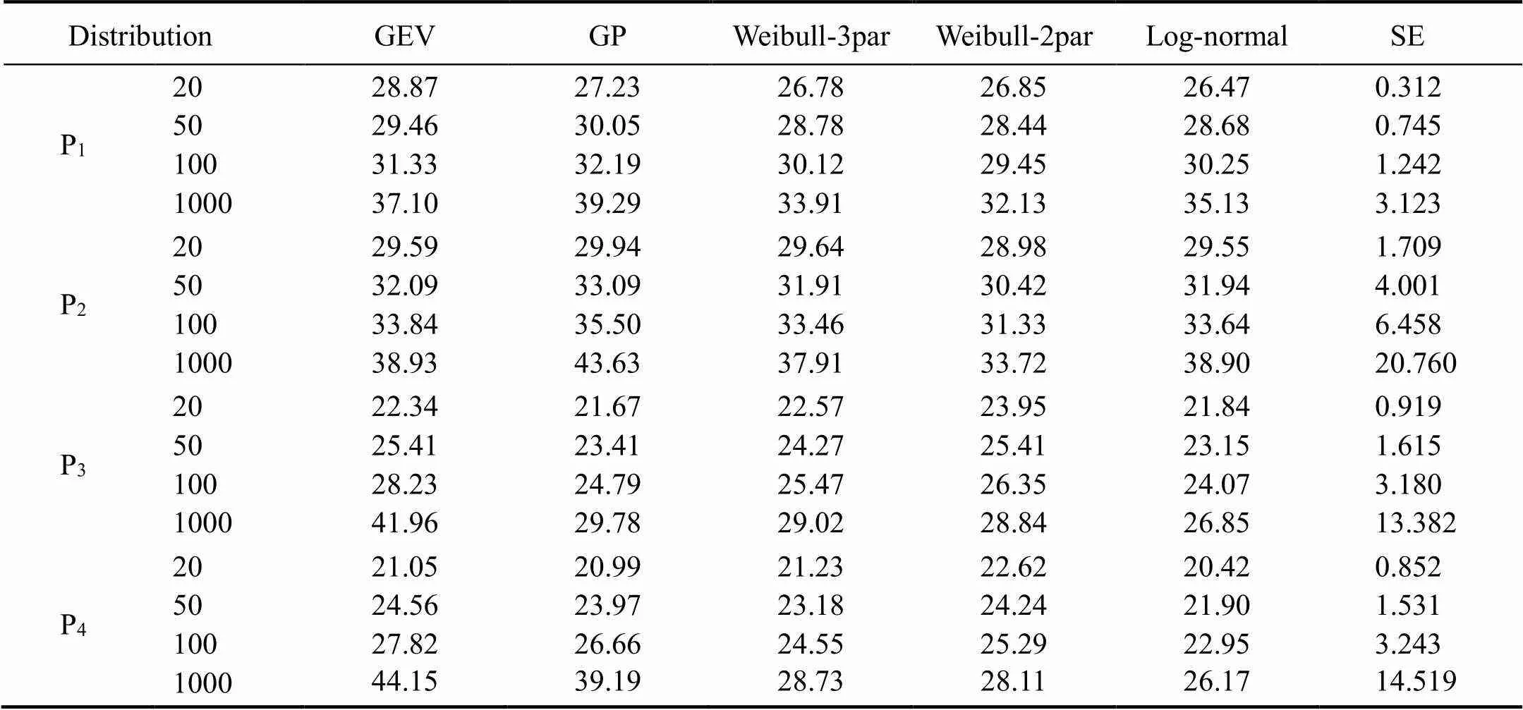
Table 4 Extreme wind speeds (ms−1) estimated using different distribution models at four sites

5.2 Monthly Extreme Wind Speed

Because P2has the best goodness of fit, this point is selected as an example to discuss the monthly extreme wind speed. Table 5 shows the calculated results using different data sets, annual maxima, and monthly maxima. Notably, the annual maxima data set produces higher results for shorter return periods and lower results for longer return periods. The SE values indicate that the difference between the two sampling methods decreases as the return period increases.

Figs.7 and 8 show that TCs occur more frequently in summer and autumn than in spring and winter. Similarly, the intensity of typhoons is stronger in summer and autumn than in spring and winter. Table 6 shows the return levels of wind speed for each month, with noticeable monthly differences. September has the highest extreme wind speed, followed by June and October; their 100-year return level values are 35.37, 31.84, and 31.60ms−1, respectively. Moreover, May, July, August, and November have values exceeding 20ms−1. The values for the rest of the months are lower than 20ms−1. The frequency of typhoons is high and the intensity of typhoons is strong in July, August, and September, with typhoon disasters occurring more often. In terms of the annual extreme wind speed, only September has a high value.

5.3 Comparison with Previous Studies

The estimated wind speed with a 100-year return pe- riod is compared with those reported in previous studies, as shown in Table 7. The table shows the extreme wind speeds of five coastal cities near the SCS, namely, Fuzhou, Xiamen, Shenzhen, Hong Kong, and Zhanjiang. The results of previous studies are obtained from a design code(Housing and GB50009-2012), Ou(2002), and Yan(2020a). The results of this study are estimated using the GEV distribution and ERA5 data sets. This study has the minimum value among the four results because the ERA5 data sets largely underpredict the wind speed near the TC center (Shao,2018), resulting in a small extreme wind speed value.

Table 5 Extreme wind speeds (ms−1) estimated using the annual and monthly maxima

Table 6 Return levels (ms−1) for each month

Table 7 Comparison of the extreme wind speeds (100-year return period) between different studies (ms−1)

Note:†Design code (Housing and GB50009-2012).

5.4 Comparison of Different Data Sets

The comparison of the annual extreme value sample distributions between the ERA5 and NCEP data sets is shown in Fig.13. The figure shows that the samples of the ERA5 and NCEP data sets at sites P1–P4are distributed similarly. The comparison of the estimated extreme wind speeds between the ERA5 and NCEP data sets is shown in Fig.14. The figure shows that the estimates obtained on the basis of the two data sets are similar when the return period is shorter than 100 years. However, the difference of the estimates becomes larger as the return period increases, particularly for results at P3and P4. This finding can be attributed to the fact that the samples of the ERA5 data sets at P3and P4are distributed in a dispersed manner, having many small and large values. Therefore, the samples are important for the estimation of a long return period.

6 Conclusions

In this study, the wind conditions in the SCS, including wind climate, wind energy, frequency of TC, and extreme wind speed, are analyzed systematically and comprehensively on the basis of the CMA and ERA5 data sets.

According to the average wind field in each month and the wind rose diagram, the wind speed and direction are analyzed in this study. Five offshore points are selected as calculated points to assess the wind energy potential. By comparing theAandCvalues, we determine that the offshore wind energy productivity increases along the coast from the southwest to the northeast. Moreover, four typical points in the SCS are selected to calculate the extreme wind speeds using the GEV, GP, Weibull-3par, Weibull-2par, and log-normal distributions. According to the goodness of fit, the GEV distribution is selected to calculate the extreme wind speeds in the entire SCS. The contour plot of extreme wind speeds is also drawn. The region around 15˚N, on the east side of the Indochina Peninsula, has the highest extreme wind speed.

The frequency of TC, including the monthly and spatial frequencies for different-intensity TCs, is analyzed. We can conclude that the period from May to October, with higher frequency and greater strength, is a prevalent typhoon season. On average, 16 TCs occur each year in the SCS, with a large number of severe tropical storms. The other types of TCs, including severe typhoons and super typhoons, have a similar frequency.

Moreover, the sensitivity of the key parameters of the calculation model is analyzed. The extreme wind speeds are calculated using different distribution models at four sites.The results indicate that the return levels of wind speed are similar when the return period is less than 100 years. By calculating the extreme wind speed in each month, we determine that only the monthly extreme value in September is higher than the annual extreme value.

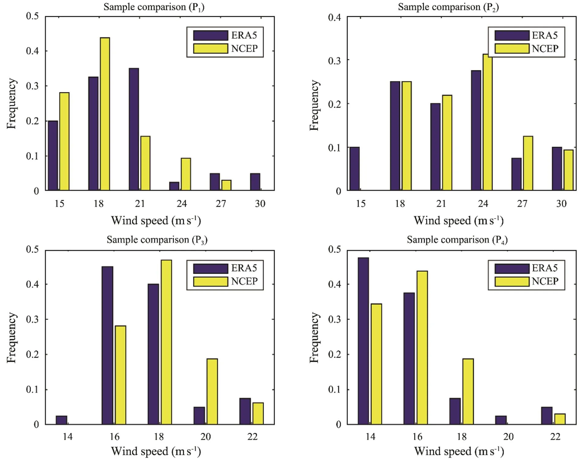
Fig.13 Comparison of the sample distribution between the ERA5 and NCEP data sets.

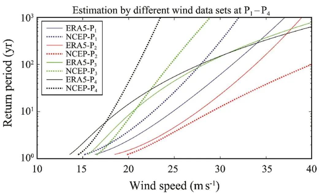
Fig.14 Comparison of the extreme wind speed estimation between the ERA5 and NCEP data sets.

Compared with the results of other studies, the estimated extreme wind speeds in this study are smaller because the extreme wind speeds in the ERA5 data sets are largely underestimated. The estimated extreme wind speeds have small differences for shorter return periods but large differences for longer return periods when different data sets are used.

Acknowledgements

This work was supported by the NSFC-Shandong Joint Fund (No. U1706226) and the Fundamental Research Funds for the Central Universities.

Ali, S., Lee, S. M., and Jang, C. M., 2018. Statistical analysis of wind characteristics using Weibull and Rayleigh distributions in Deokjeok-do Island–Incheon, South Korea.,123: 652-663.

Campos, R. M., and Soares, C. G., 2018. Spatial distribution of offshore wind statistics on the coast of Portugal using regional frequency analysis., 123: 806-816.

Cannon, D. J., Brayshaw, D. J., Methven, J., Coker, P. J., and Lenaghan, D., 2015 Using reanalysis data to quantify extreme wind power generation statistics: A 33 year case study in Great Britain., 75: 767-778.

Chen, X., Zheng, C., Zuo, C., Du, X., and Huang, Y. H., 2020. The establishment of the monthly frequency indexes of typhoon during active seasons and its application., 59 (3): 394-400 (in Chinese with English abstract).

Chidean, M. I., Caamaño, A. J., Ramiro-Bargueño, J., Casanova-Mateo, C., and Salcedo-Sanz, S., 2018. Spatio-temporal analysis of wind resource in the Iberian Peninsula with data-coupled clustering., 81: 2684-2694.

Gao, H., Wang, L., Liang, B., and Pan, X., 2018. Estimation of extreme significant wave heights in the Yellow Sea, China.. Sapporo, 387-391.

GB50009-2012, 2012. Load code for the design of building structures. Ministry of Housing and Urban-Rural Development of the People’s Republic of China, 1-10.

Geyer, B., Weisse, R., Bisling, P., and Winterfeldt, J., 2015. Climatology of North Sea wind energy derived from a model hindcast for 1958–2012., 147: 18-29.

Haghroosta, T., and Ismail, W. R., 2017. Typhoon activity and some important parameters in the South China Sea., 17: 29-35.

Hasager, C. B., Mouche, A., Badger, M., Bingöl, F., Karagali, I., Driesenaar, T.,, 2015. Offshore wind climatology based on synergetic use of Envisat ASAR, ASCAT and QuikSCAT., 156: 247-263.

Haver, S., and Winterstein, S. R., 2009. Environmental contour lines: A method for estimating long term extremes by a short term analysis., 116: 116-127.

Kantar, Y. M., Usta, I., Arik, I., and Yenilmez, I., 2018. Wind speed analysis using the extended generalized Lindley distribution., 118: 1024-1030.

Lee, B. H., Ahn, D. J., Kim, H. G., and Ha, Y. C., 2012. An estimation of the extreme wind speed using the Korea wind map., 42: 4-10.

Liang, B., Shao, Z., Li, H., Shao, M., and Lee, D., 2019. An automated threshold selection method based on the characteristic of extrapolated significant wave heights., 144: 22-32.

Liu, D., Han, F., Pang, L., Li, H., Xie, B., and Wang, F., 2010. Probabilistic approach of coastal defense against typhoon attacks for nuclear power plant., 24 (2): 265-275.

Liu, D., Wang, L., and Pang, L., 2006. Theory of multivariate compound extreme value distribution and its application to extreme sea state prediction., 51 (23): 2926-2930.

Lombardo, F. T., Main, J. A., and Simiu, E., 2009. Automated extraction and classification of thunderstorm and non-thunderstorm wind data for extreme-value analysis., 97 (3-4): 120-131.

Nedaei, M., Assareh, E., and Biglari, M., 2014. An extensive evaluation of wind resource using new methods and strategies for development and utilizing wind power in Mah-shahr station in Iran., 81: 475-503.

Niroomandi, A., Ma, G., Ye, X., Lou, S., and Xue, P., 2018. Extreme value analysis of wave climate in Chesapeake Bay., 159: 22-36.

Ohunakin, O. S., and Akinnawonu, O. O., 2012. Assessment of wind energy potential and the economics of wind power generation in Jos, Plateau State, Nigeria., 16 (1): 78-83.

Ou, J., Duan, Z., and Chang, L., 2002. Typhoon risk analysis for key coastal cities in Southeast China., 11 (4): 9-17.

Pang, L., Liu, D., Yu, Y., and Jiang, J., 2007. Improved stochastic simulation technique and its application to the multivariate probability analysis of typhoon disaster.. Lisbon, 1800-1805.

Shao, Z., Liang, B., Li, H., Wu, G., and Wu, Z., 2018. Blended wind fields for wave modeling of tropical cyclones in the South China Sea and East China Sea., 71: 20-33.

Shi, Y., Du, Y., Chen, Z., and Zhou, W., 2020. Occurrence and impacts of tropical cyclones over the southern South China Sea., 40 (9): 4218-4227.

Tizpar, A., Satkin, M., Roshan, M. B., and Armoudli, Y., 2014. Wind resource assessment and wind power potential of Mil-E Nader region in Sistan and Baluchestan Province, Iran–Part 1: Annual energy estimation., 79: 273-280.

Wang, J., Qin, S., Jin, S., and Wu, J., 2015. Estimation methods review and analysis of offshore extreme wind speeds and wind energy resources.,42: 26-42.

Wang, X., and Zhao, W., 2019. Characteristics analysis of wind and wave in the Nansha Area based on ERA-Interim reanalysis data., 36 (2): 30-37 (in Chinese with English abstract).

Wang, Z., Duan, C., and Dong, S., 2018. Long-term wind and wave energy resource assessment in the South China Sea based on 30-year hindcast data., 163: 58-75.

Weisser, D. A., 2003. Wind energy analysis of Grenada: An estimation using the ‘Weibull’ density function., 28 (11): 1803-1812.

Wu, G., Shi, F., Kirby, J. T., Liang, B., and Shi, J., 2018. Modeling wave effects on storm surge and coastal inundation., 140: 371-382.

Wu, G., Wang, J., Liang, B., and Lee, D. Y., 2014. Simulation of detailed wave motions and coastal hazards., 72: 127-132.

Yan, Z., Liang, B., Wu, G., Wang, S., and Li, P., 2020a. Ultra-long return level estimation of extreme wind speed based on the deductive method., 197: 106900.

Yan, Z., Pang, L., and Dong, S., 2020b. Analysis of extreme wind speed estimates in the northern South China Sea., 59 (10): 1625-1635.

Yan, Z., Wu, G., Liang, B., and Li, P., 2020c. a stochastic tropical cyclone model for the northwestern Pacific Ocean with improved track and intensity representations., 105: 102423.

Yang, J., Liu, Q., Li, X., and Cui, X., 2017. Overview of wind power in China: Status and future., 9 (8): 1454.

Yao, Z., Xiao, J., and Jiang, F., 2012. Characteristics of daily extreme-wind gusts along the Lanxin Railway in Xinjiang, China., 6: 31-40.

Ying, M., Zhang, W., Yu, H., Lu, X., Feng, J., Fan, Y.,, 2014. An overview of the China Meteorological Administration tropical cyclone database., 31 (2): 287-301.

Young, I. R., and Donelan, M. A., 2018. On the determination of global ocean wind and wave climate from satellite observations., 215: 228-241.

Zheng, C. W., and Pan, J., 2014. Assessment of the global ocean wind energy resource., 33: 382-391.

Zheng, C. W., Liang, F., Yao, J. L., Dai, J. C., Gao, Z. S., Hou, T. T.,, 2020. Seasonal extreme wind speed and gust wind speed: A case study of the China Seas., 99 (SI): 435-438.

Zheng, C. W., Pan, J., and Li, J. X., 2013. Assessing the China Sea wind energy and wave energy resources from 1988 to 2009., 65: 39-48.

Zheng, C. W., Xiao, Z. N., Zhou, W., Chen, X. B., and Chen, X., 2018.. Springer Nature, Singapore, 1-10.

Zheng, C. W., Zhuang, H., Li, X., and Li, X., 2012. Wind energy and wave energy resources assessment in the East China Sea and South China Sea., 55 (1): 163-173.

October 14, 2020;

November 18, 2020;

May 27, 2021

© Ocean University of China, Science Press and Springer-Verlag GmbH Germany 2022

#The two authors contributed equally to this work.

. E-mail: pang@ouc.edu.cn

(Edited by Xie Jun)