A new approach for accurate determination of particle sizes in microfluidic impedance cytometry

N.Priyadarshi, U.Abbasi, V.Kumaran, and P.Chowdhury

ABSTRACT In microfluidi impedance cytometry,the change in impedance is recorded as an individual cell passes through a channel between electrodes deposited on its walls,and the particle size is inferred from the amplitude of the impedance signal using calibration.However,because the current density is nonuniform between electrodes of finit width,there could be an error in the particle size measurement because of uncertainty about the location of the particle in the channel cross section.Here,a correlation is developed relating the particle size to the signal amplitude and the velocity of the particle through the channel.The latter is inferred from the time interval between the two extrema in the impedance curve as the particle passes through a channel with cross-sectional dimensions of 50μm(width)×30μm(height)with two pairs of parallel facing electrodes.The change in impedance is predicted using 3D COMSOL finite-elemen simulations,and a theoretical correlation that is independent of particle size is formulated to correct the particle diameter for variations in the cross-sectional location.With this correlation,the standard deviation in the experimental data is reduced by a factor of two to close to the standard deviation reported in the manufacturer specifications

KEYWORDS Impedance cytometry,Lab on chip,COMSOL simulation

I.INTRODUCTION

Single-cell impedance cytometry is becoming a widely used noninvasive method for determining the properties of cells,such as their sizes,shapes,and dielectric properties.1The size of a single cell was firs determined by Coulter2via DC resistance measurement.More recently,AC methods have been used to determine both the size and properties of the cell membrane,such as cytoplasm and subcellular components.3–8In general,impedance cytometry of a cell is carried out in a microfluidi channel based on the impedance signal when the cell—suspended in a conductive solution—passes through microelectrodes fabricated on the inner walls of the channel,and accurate determination of particle size has been explored with different microelectrode configurations9–12

The literature contains two different microelectrode configura tions,i.e.,(i)coplanar,where the electrodes are etched on one wall of the channel with rectangular cross section,and(ii)parallel facing,where the electrodes are located on opposite walls of the channel.A microfluidi chip with a coplanar configuratio is a relatively cheap device that is easy to fabricate.However,as the cross-stream distance of the particle from the nearest electrode surface increases,the measured signal amplitude decreases,and this limits the range of particle size for a particular channel configuration in a channel with a height of tens of micrometers,the minimum particle size that can be detected is～2μm.By contrast,with parallel facing electrodes,the impedance depends on only the perpendicular distance of the particle from the nearest electrode surface,increasing as that distance decreases.However,the fabrication procedure is more complicated because it requires accurate alignment of the electrodes on opposite walls.13

Recently,the coplanar configuratio was used to measure the diameters of submicrometer particles.1,14–16De Ninno et al.14demonstrated accurate size determination of particles with diameters of 5.2μm and above by using fiv electrodes in a microchannel with cross-sectional dimensions of 40μm(width)×21μm(height)and with the addition of floatin electrodes;the impedance signal involved an additional parameter known as relative prominence,which was used to correct the particle diameter with a resolution of 0.3μm,where the resolution is define as the difference in particle size corresponding to twice the standard deviation of the distribution.Using double differential electrodes in the coplanar configuration Zhong et al.15measured particle size with a resolution of 0.1μm,but the channel dimensions were restricted to 8μm(width)×10μm(height),and such small channels are susceptible to clogging.Several studies have used parallel electrodes to determine particle diameters,1,17–19and in most cases particle diameters of 3–10μm were studied with a resolution of 1μm.

Irrespective of the electrode configuratio in the microchannel,the differential signal amplitude generated by a particle as it passes the electrodes depends on its perpendicular distance from them.Known as position dependency,this phenomenon results in significan errors in diameter measurements,and various approaches have been used to understand the position dependency of the signal amplitude and correct for it.14,16,17Spencer et al.17measured both transverse and oblique signal amplitudes simultaneously by using multiple pairs of electrodes to determine the transit times of particles,and the relative values of these transit times were used to correct for the position dependency in the direction perpendicular to the electrode surface.The signals measured using three pairs of coplanar electrodes were fitte using a bipolar Gaussian equation,and shape parameters obtained from this fi varied with both particle position and diameter,allowing correction for position dependency.However,because the coplanar configuratio is more sensitive to measurement inaccuracy due to position dependency,using it to quantify smaller particle diameters is considered infeasible.

Herein,we propose a method involving three pairs of parallel facing electrodes to improve the estimation of particle diameter.By extracting both peak amplitude and travel time from the measured signal traces and the theoretically simulated curves,this method provides a simple strategy for correcting for particle position dependency.The novelty of the present work stems from the choice of travel time,for which a general strategy is introduced.17,20

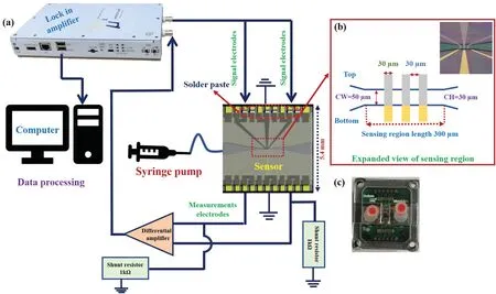
FIG.1.Complete setup for impedance measurements of beads suspended in phosphate-buffered saline solution.

II.EXPERIMENTAL METHODS

The experimental setup is shown schematically in Fig.1(a).A microfluidi chip with dimensions of 5.4 mm×5.4 mm with parallel facing electrodes was fabricated on a two-inch wafer using our in-house facilities.The top and bottom walls for the electrodes were made of Si/SiO2and glass,respectively.As shown in Fig.1(b),the configuratio comprised a microfluidi channel with cross-sectional dimensions of 50μm(width)×30μm(height).On the top and bottom walls of the channel were three pairs of electrodes,each electrode with a width of 30μm and separated by an edge-to-edge distance of 30μm.The electrical circuit is shown in Fig.1(a),and the center electrodes on the top and bottom walls were grounded.

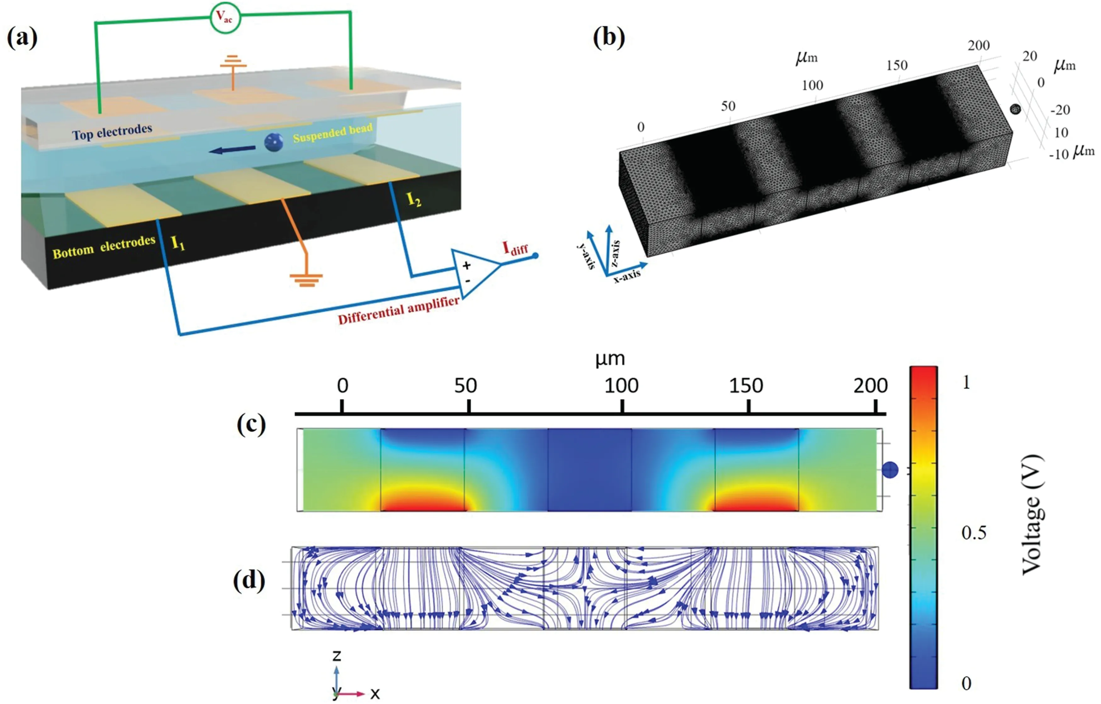
FIG.2.(a)Channelconfiguration showing(i)particle traveling in channelwith cross-sectionaldimensions of 30μm×50μm,(ii)top and bottom electrodes,(iii)applied voltage,and(iv)outputcurrent.(b)Mesh used in typical3D COMSOL simulations for a particle with a diameter of3μm,highlighting the higher meshing density atthe electrodes.(c)and(d)Potentialand currentdensity distributions in xz plane of channelwith an applied voltage of1 V.

The Cr/Pt/Au electrodes(20 nm/150 nm/100 nm)were deposited on both the Si/SiO2and glass substrates,and the desired electrode pattern as shown in Fig.1(b)was fabricated using optical photolithography and ion milling.The channel fabrication and bonding were done using a photoimageable resist(Perminex 2015,USA)and a bonding chuck as per the manufacturer data sheet.See our previous work21for the details of fabricating the sensor.Using an existing semiconductor facility,the electrical contacts were wirebonded to a printed circuit board and connected to male header pins for direct coupling with the female sockets;this was possible by an innovative change in our design,with the top electrode contacts accessible through the bottom electrodes by fillin the gap with fin solder paste(Chip Quik-SMD291SNL T7,USA).Side holes for flui access were injected with transparent flui connectors that were glued using UV glue(Bondic,USA)directly on the chip.A photograph of the fabricated lab-on-a-chip is shown in Fig.1(c).The inlet of the flui connector was then connected to a syringe pump via a Teflo tube(inner diameter:0.3 mm;outer diameter:0.8 mm).

Polystyrene beads with a density of 1.05 g/cm3,a DC conductivity of 6.6×10−4S/m,and diameters of 2μm,3μm,4μm,5μm,and 6μm(Lab261,1%solid)were used for the measurements.They were suspended in phosphate-buffered saline(PBS)with a DC conductivity of 1.6 S/m and diluted to a concentration of～200 beads per microliter.The carrier signal applied to the top electrodes had a frequency of 1.8 MHz and a peak-to-peak amplitude of 7.5 V.The currents from the bottom left and right electrodes were converted to a voltage difference using transimpedance operational amplifier(THS 4303)in which the inverting inputs were grounded.The outputs of the two transimpedance amplifier were connected to the input of a differential amplifie(ADA4927),which provided the voltage difference between the two electrodes.At constant voltage,the current is inversely proportional to the impedance,and the results herein are expressed in terms of the impedance.As a cell passes sequentially past the left and right electrodes,the difference in impedance is positive when the particle is between the upstream pair of electrodes and then becomes negative when it passes through the downstream pair.

The impedance measurements of the fast-moving cells suspended in the PBS solution required a high sampling rate.The fastest-moving cells in the channel with cross-sectional dimensions of 50μm×30μm at a flo rate of 30μl/min travelled at 0.7 m/s,and the time to cross the electrode zone of length 150μm was～0.2 ms.Therefore,a sampling rate of 350 000 samples per second provided～75 measurements within the time taken for a cell to cross the electrode zone,which was sufficien to capture the signal with no distortion.The current lock-in amplifie designed by MicroX could generate three different frequencies in a single channel ranging from 10 kHz to 15 MHz and also had the in-built feature of real-time data processing for event counting by a custom-made algorithm programmed in the digital signal processor integrated in the lock-in board.The demodulated data from the lock-in amplifie were transferred to computer memory through a universal serial bus and were recorded in binary format.The frequency generation,low-pass-filte cut-off frequency,and sampling rate were controlled using an application programming interface made for a Linux-based system.The front-end electronics shown in Fig.1 had precision resistors of 1 kΩ with a tolerance of less than 0.05%,and these were used to set the required gain of the differential amplifier

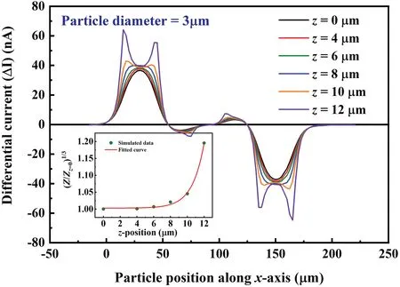
FIG.3.Differential currentΔI versus particle position along x direction of microchannelfor different z positions perpendicular to electrodes.The insetshows the maximum impedance at different z locations scaled by the impedance at the center ofthe channelat z=0.

FIG.4.(a)Velocity profile for a 30μm(height)×50μm(width)channelobtained from COMSOL simulation(verified using analyticalsolution).(b)Normalized impedance as a function of velocity normalized with maximum velocity at y=z=0.

III.THEORETICAL ANALYSIS

Electric-fiel simulations were carried out using the COMSOL 5.6 finite-elemen solver,and the analytical solution for a single pair of electrode was reported earlier.22The potential V in the flui and particle is governed by the Laplace equation∇2V=0.The boundary condition of zero potential gradient was applied at the top and bottom surfaces of the channel,i.e.,n⋅∇V=0,because these surfaces are considered to be insulating;here,n is the unit normal to the surface.The boundary condition of constant potential was applied at the electrode surfaces.Because the boundary condition changes discontinuously at the junction between a bare channel wall and an electrode deposited thereon,the fiel lines have large curvature near the electrodes,and because of this,it was necessary to refin the mesh near the electrodes as shown in Fig.2(b).In total,2×106mesh points were used in a typical simulation configuratio of the type shown in Fig.2(b).Distributions of potential and current density across the channel with an applied voltage of 1 V are shown in Fig.2(c).

Simulation results for the change in current due to a particle with a diameter of 3μm are shown in Fig.3,where the impedance is shown as a function of downstream distance at different z locations in the direction perpendicular to the top and bottom walls.Even for the same particle size,the impedance curves differ significantly in shape depending on the z position of the particle.In each case,there are at least four extrema as the particle passes through the channel.When it passes through the center of the channel,the current changes relatively smoothly and can be fitte well by Gaussian curves.When the particle is close to a wall,there are two maxima in the current when the particle crosses the left and right edges of each electrode,and the amplitude deviates from single Gaussian behavior with two sharp peaks near the edges of the electrodes.17

To understand the position dependency of the peak amplitude,the maximum from each set of curves for different z values was extracted and then normalized by the impedance at the center of the channel at z=0[Z/Z0∝ΔImax(z)/ΔImax(0)].Here,the maximum of the time trace of the impedance is used for bimodal curves,and Z0is the maximum impedance measured at z=0.The fitte curve in the inset of Fig.3(b)shows that the maximum amplitude changes exponentially as a function of vertical position.

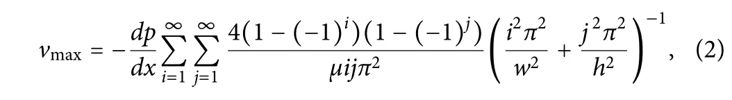
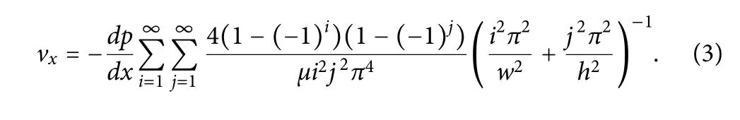
A series solution can be obtained for the flui velocity profil for the flo in a rectangular channel by using separation of variables.The velocity depends on the pressure gradient dp/dx along the channel:23

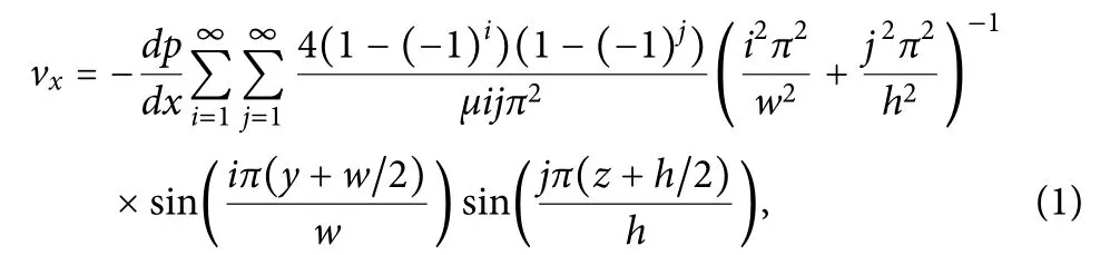
where−h/2≤z≤h/2 is the direction perpendicular to the electrodes,and−w/2≤y≤w/2 is that perpendicular to the flo direction and parallel to the electrodes.The maximum velocity at the center of the channel at y=z=0 is

and the average velocity vavis

Although the velocity profil in 3D space is an inverted paraboloid(not shown here),for y=0 it becomes a parabola as shown in Fig.4(a),which can be fitte using

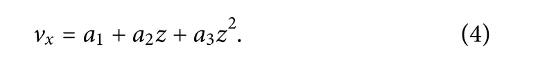
At the experimental flo rate of 30μl/min,the value of vmaxat the center was 0.68 m/s,and for this maximum velocity,the coefficient a1,a2,and a3for the parabolic fi in Fig.4(a)are 0.68 m/s,−1.13×10−5s−1,and−0.003 m−1s−1,respectively.

Because the particle position and size are unknown,the velocity is used as a parameter for correcting the particle size.The velocity is inferred from the time taken by the particle to travel from one electrode pair to the next.Although the maximum impedance is independent of the y position,the maximum velocity in a horizontal plane at a fixe z location does depend on the horizontal cross-stream coordinate y.Here,the maximum velocity vmaxat the channel center at y=z=0 is used as the normalizing factor.

The variation of Z/Z0versus vx/vmaxat y=0 is shown in Fig.4(b),and the following provides a good fi for this curve:

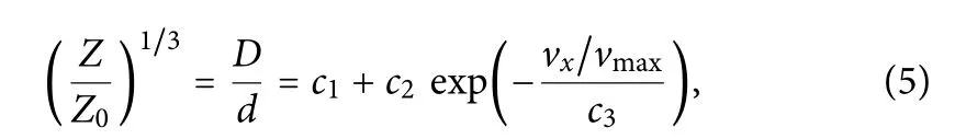
where d is the corrected diameter,D is the electrical diameter,and c1,c2,and c3are the fittin constants.The curve fittin was done using cftool in MATLAB,using the linear least-squares method known as the Levenberg–Marquardt algorithm to obtain a minimum R2=99%.

For the present experimental system,the electrical diameter D is define as

where G is the amplificatio factor to account for the currentto-voltage converter board and other electronic peripherals to be calibrated from experimental data.The value of G was estimated as 73.5μm(nA)(−1/3)using the assumption that the true diameter and the electrical diameter are equal for particles moving at the center of the channel with maximum velocity.Equation(5)allows the corrected diameter to be determined once the values of D and the particle velocity vxare known.

FIG.6.(a)Scatter plotof velocity versus electricaldiameter for 2-μm particles from separate runs,showing clearly the instrument resolution of up to 1.7μm.(b)Histogram of corrected diameter of 2-μm particles.(c)and(d)Color density plots of velocity versus electricaland corrected diameter,respectively.

IV.RESULTS AND DISCUSSION

Figure 5 shows time traces of impedance measurements with sampling at intervals of 3.3μs for particles with a diameter of 3μm.Figure 5(a)shows that the peak amplitude of Z/Z0is in the range of 1%–1.75%,which corresponds to variation of the electrical diameter D by 20%.This agrees well with the theoretical prediction as shown in the inset of Fig.3.Figures 5(b)–5(e)show expanded time traces of the impedance as a single particle travels through the channel.The velocities inferred from the time interval between two extrema are 0.54 m/s,0.49 m/s,0.36 m/s,and 0.28 m/s,respectively,and the values of the electrical diameter D derived using Eq.(5)are 3.05μm,3.35μm,3.45μm,and 3.71μm,respectively.From these figures it is clear that the shapes of the impedance trajectories of particles moving with different velocities corresponding to different z positions agree qualitatively with the theoretical predictions shown in Fig.3.As the velocity decreases,the particles are located closer to the electrodes,and the impedance trajectory has a bimodal Gaussian shape.

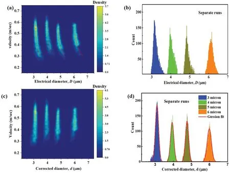
FIG.7.Separate runs with different particle sizes:(a)and(b)electrical-diameter histogram for particles ofdifferent sizes,and corresponding correction in histogram shape;(c)and(d)scatter plot of velocity versus electricaldiameter for different particle sizes,and corresponding change in plot due to size correction.

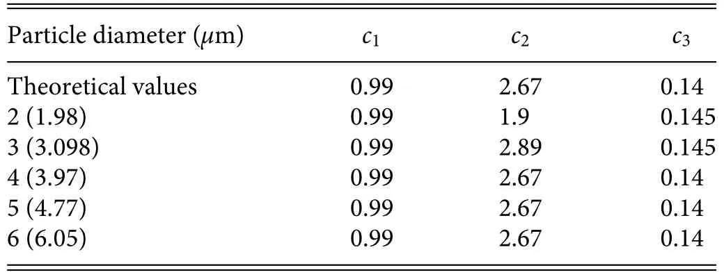
TABLE I.Parameters used to fitdata in Figs.5 and 6.

Figure 6(a)is a scatter plot of velocity versus electrical diameter D for particles with a diameter of 2μm.This shows clearly that the instrument resolution was～1.7μm,and there was electrical noise for electrical diameters below this value.The maximum measured particle velocity vmaxwas～0.67 m/s,which is very close to the theoretically predicted value of～0.68 m/s for the aforementioned channel dimensions and flo rate.The increase of D signifie the position dependency of the particle in the z direction as shown in Fig.6(c).Using Eq.(5),the corrected particle diameter d was derived for the whole population of data;the corresponding histogram plot is shown in Fig.6(b),and a color density plot of velocity versus d is shown in Fig.6(d).These show a significan narrowing of the distribution and a reduction in the coefficien of variation,with the particle size now independent of velocity.The values of the coeffi cients c1,c2,and c3used in Eq.(5)were obtained from the theoretical results given in Table I.

The density of sampling points is shown in the electricaldiameter–velocity plane in Fig.7 for particles with average diameters of～3.0μm,4.0μm,5.0μm,and 6.0μm.For all diameters,the density plot in particle-diameter–velocity space[Fig.7(a)]shows a systematic variation of the electrical diameter with velocity,which is a consequence of the position dependence of the impedance in the z direction.Applying Eq.(5)to all the individual populations reduces the standard deviation in the distributions for all sizes,and the particle size is now independent of velocity.Figure 7(b)shows that the histogram of the uncorrected diameter is an asymmetric Gaussian distribution with a relatively large standard deviation.When Eq.(5)is applied,the distribution shown in Fig.7(d)is closer to a symmetric Gaussian with a smaller standard deviation.From these plots,it is inferred that the correlation used to correct the electrical diameter works effectively for all particle sizes with the same fittin constants.

Figure 8 shows similar plots for experiments with a mixture of beads.Figure 8(a)shows that regardless of particle size,the ratio D/d varies in a similar manner with velocity.Figure 8(b)shows that the histogram of the uncorrected diameter is an asymmetric Gaussian distribution and for each particle diameter,the distribution width is large.The electrical diameter was corrected using Eq.(5)with the same values for c1,c2,and c3as those in the simulations for all particle sizes.There is a significan reduction in the spread of the histograms for particles of different sizes as shown in Figs.8(c)and 8(d),and the comparative results are provided in Table II for different particle sizes.From Table II,for the separate runs it is clear that there was a reduction in the standard deviation by a factor of two irrespective of particle diameter,which indicates the validity of the empirical relationship in Eq.(5).The experimental data from the mixed runs show again the applicability of Eq.(5),where both the standard deviation and coefficien of variation(CV)were found to be of the same orders of magnitude as those estimated from the separate runs.The estimated CV for each particle diameter was found to be very close to that from the manufacturer;the exception was that for the diameter of 3μm,for which the CV provided by the manufacturer is very low compared to those for the other diameters.

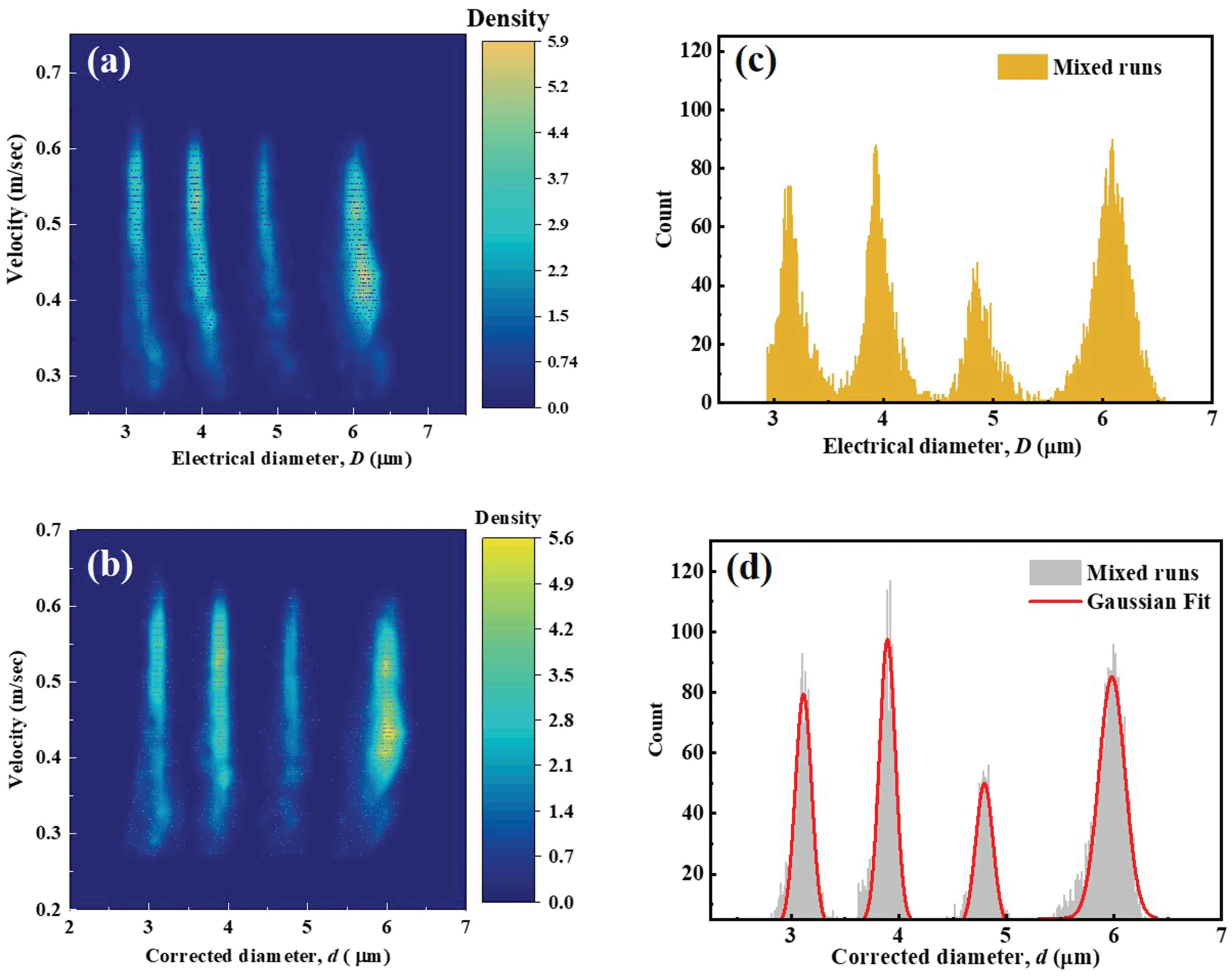
FIG.8.Mixed runs with different particle sizes:(a)and(b)electric-diameter histogram,and corresponding correction in histogram shape;(c)and(d)scatter plot of velocity versus electricaldiameter for mixed runs,and corresponding plot with correction.

TABLE II.Comparison between statisticaldata provided by manufacturer and those obtained before and after corrections were applied to the experimentaldata.

V.CONCLUSION

An important difficult in determining the diameter of a particle of micrometer size by using impedance measurements in a microchannel is the uncertainty about its location in the channel cross section.For a particle of given size,the measured impedance is higher if the particle is closer to the electrodes and lower when it is in the center of the channel.Because of this,the electrical diameter inferred from impedance measurements has a significan error when compared to the true diameter.Herein,a procedure was formulated for correcting the electrical diameter to obtain the true diameter.The particle velocity is used as a single parameter to represent the variation in position in the cross section,and the ratio of the electrical and true diameters is expressed as a three-parameter fi[Eq.(5)].Although the velocity depends on the two cross-stream coordinates whereas the impedance correction depends on only the coordinate perpendicular to the electrodes,we found a very good correlation between the velocity and the correction to the diameter using the three-parameter fit There is a reduction by a factor of two in the standard deviation of the measured particle diameter by using this empirical correlation.

Surprisingly,we also found that the coefficient in Eq.(5)are independent of the particle diameter.The same coefficient were found to minimize the standard deviation in particle size for particles with diameters of 2–8μm.This indicates that the coefficient are functions of only the channel and electrode configuration and do not depend on the size of the particle in the channel.Therefore,once the coefficient have been calibrated for one particle size for a given channel configuration they can be used for other particle sizes.This provides a robust method for correcting the particle size for variations in cross-sectional location for samples in which the particle size distribution is discrete,so that the spread in the size distribution is smaller than the difference in the discrete size ranges.A more sophisticated procedure is being developed for size correction when there is a continuous size distribution.

ACKNOWLEDGMENTS

The authors would like to thank(i)the Director of CSIR–NAL for supporting this activity and(ii)the Polish grant committee for funding the“Bridge Alpha”grant for this project.

AUTHOR DECLARATIONS

Conflict of Interest

The authors have no conflict to disclose.

DATA AVAILABILITY

The data that support the finding of this study are available from the corresponding author upon reasonable request.