基于DRASTIC- LU参数和数据驱动模型的地下水硝酸盐脆弱性分区

Seyed Ahmad Eslaminezhad, Mobin Eftekhari, Mohammad Akbari

(1.德黑兰大学工程学院测绘与地理信息工程系， 伊朗 德黑兰 1417466191；2.伊斯兰阿扎德大学马什哈德分校土木工程系， 伊朗 马什哈德 9187147587；3.比尔詹德大学土木工程系， 伊朗 比尔詹德 9717434765)

1 研究背景

现代社会对自然资源的过度使用和污染物的大量排放已经威胁到地下水资源并造成严重污染. 自然和人为污染过程已导致全球的水质迅速下降，在发展中国家尤为严重[1]. 当前，地表水和地下水污染有关问题的水质调查广泛展开[2]. 由于含水层中污染物容量高、持续时间长和自然净化弱，一旦含水层受到污染，污染将持续存在[3-4]. 此外，改善地下水质量的含水层净化是一个复杂的过程，需要时间和资金. 因此，控制或减少地下水污染是地下水资源管理的重要原则之一[5]. 1960年法国学者首次提出脆弱性的概念. 脆弱性是一种相对属性，无法察觉和测量，取决于地质和水文地质环境的含水层特性[6]. 为了评估脆弱性，已经提出多种方法，包括基于过程的评价法、统计方法和重叠评价法[7]. 其中，基于过程的评价法利用仿真模型来估计污染物的运移；统计方法分析地下水空间变量与污染物量之间的相关性；重叠评价法综合考虑污染物从地表运移到地下饱水区的控制参数，并计算一个区域不同部分的脆弱性指数[7]. 最著名的重叠指数方法之一是Aller等[8]在1987年为美国环境保护署开发的DRASTIC模型，该模型将通过不同参数获得的信息利用地理信息系统(geographic information system,GIS)进行组合分析. DRASTIC模型基于水文地质概念，将特定区域的物理和水文地质特征相结合[9]. 本文DRASTIC- LU模型的主要优点之一是使用多个信息层进行脆弱性评估，减少了错误信息或难以预料问题对最终结果的影响[10]. 此外，本文的模型比基本的DRASTIC模型具有更多的土地利用层[10]. DRASTIC- LU模型包括含水层埋深、净补给量、含水层介质、土壤介质、地形、渗流带的影响、水力传导率和土地利用等参数. 根据前人的研究，地下水脆弱性图绘制分析可以分为知识驱动和数据驱动两大类方法[1,11]. 数据驱动的方法对于研究充分区域或统计数据数量(参考数据)足够的区域非常有效，该方法目的是确定更详细的工作位置. 知识驱动的方法对于初步研究地区、目标或数据很少的区域有效. 权重估计和分类估计是基于专家的判断，不需要已知的数据. 基于知识驱动和数据驱动集成方法在地下水脆弱性图中已有大量研究，仅举几例：

Sener等[1]建立了基于Egirdir湖流域的GIS的DRASTIC模型. 在本案例研究中，使用DRASTIC和DRASTIC- AHP模型做出地下水脆弱性图，并用于线性回归来确定地下水脆弱性(硝酸盐质量浓度)与含水层脆弱性区域之间的关系. 研究结果表明，与DRASTIC模型相比，DRASTIC- AHP模型与该区域的硝酸盐质量浓度具有更大的相关性. Pisciotta等[2]使用SINTACS模型和DRASTIC模型评估地下水中硝酸盐污染的内在脆弱性，并比较意大利地中海地区西西里岛农业过度发展带来的环境影响. 通过皮尔逊相关方法将获得的硝酸盐质量浓度值与SINTACS和DRASTIC值进行比较，结果表明SINTACS模型与硝酸盐质量浓度值具有更大的相关性. Khan等[6]使用DRASTIC模型、改进的DRASTIC- LU模型、DRASTIC- AHP模型和改进的DRASTIC- LU- AHP模型来评估Raipur市的地下水脆弱性. 他们使用这4个模型将地下水脆弱性分为非常低、低、中等、高和非常高5个类别. 为了确定DRASTIC模型的准确性，总共使用了50个季风前和季风后季节的硝酸盐质量浓度的地下水样，并发现改进的DRASTIC- LU- AHP模型最准确并且最适合该研究区域. Chamanehpour等[12]使用DRASTIC模型、SINTACTS模型和FUZZY- DRASTIC模型评估Nehbandan市地下水固有脆弱性. 研究结果表明，评估该地区地下水脆弱性的最佳方法是FUZZY- DRASTIC模型，该模型与该地区硝酸盐质量浓度的相关系数高于DRASTIC和SINTACS模型. Koh等[3]使用普通最小二乘(ordinary least squares,OLS)回归和地理加权回归(geographically weighted regression,GWR)方法来确定整个岛屿硝酸盐质量浓度与各种参数(地形、水文和土地利用)之间的关系. 比较OLS模型和GWR模型发现， GWR模型比OLS模型能更好地反映地下水脆弱性. 这项研究的结果证明，GWR模型是研究地下水质量与环境因素之间不同空间关系的有效工具.

迄今为止，地下水脆弱性图的制作受到广泛关注，但是在对其进行的研究中，有一些问题没有被充分关注. 首先，这些研究都没有为地下水脆弱性分区提供足够的参数组合. 其次，尚未使用适当的分析来确定有效DRASTIC- LU参数的最佳组合，并基于有效DRASTIC- LU参数做出地下水脆弱性分区图. 本研究中，通过改进的DRASTIC模型(将土地利用图添加到模型中)，除了确定Birjand平原含水层对污染的脆弱性外，还考虑地下水资源管理中影响含水层脆弱性的最有效参数. 因此，为了达到本研究的目的，根据该地区硝酸盐质量浓度(参考数据)的适合性，结合空间和非空间数据驱动方法，包括人工神经网络(artificial neural network,ANN)和GWR结合二元粒子群算法(binary particle swarm optimization,BPSO)，在确定有效DRASTIC- LU参数的最佳组合的基础上，制作地下水脆弱性图.

2 方法

2.1 研究区域

研究区域为Birjand，位于Bagheran高地的北部，经度为59°13′，纬度为32°53′. 该平原近似长方形状，北至Moli高地和Markooh城堡，南至 Bagheran高地和Rach山，东至Bandar山和Amin Abad村庄，西至Korang和Chang高地，并在其中心区域形成冲积含水层. Birjand平原含水层补给区的总面积约为3 425 km2，其中980 km2是平原，其余为高地. 年平均降水量为170 mm，Birjand平原的最高和最低海拔分别为1 491 m和1 295 m. 该地区的土地包括旱地、荒地、农田和居民区. Birjand含水层的形状几乎为矩形，平均长度为55 km，宽度为5 km[13]. 图1为本研究中数学方法的流程图.

图1 本研究的数学方法流程

2.2 DRASTIC- LU模型

DRASTIC模型用于利用水文地质参数评估地下水相对污染脆弱性的能力. 该模型由7个可测量的水文地质参数组合而成，这些参数影响污染物运移到地下水中，这些参数包括含水层埋深、净补给量、渗流层影响、土壤介质、含水层介质、水力传导率和地形. 在本研究中，增加了土地利用层以提高模型的准确性.

地表和地下水位之间的距离称为含水层埋深，表示污染物到达地下水必须经过的深度，m[14]. 净补给量指从地表渗入地下水位的水量，mm/a[15]，此外，通过增加某个地区的净补给量，该地区的地下水污染潜力将会增加. 渗流层指地下水位和非饱和土壤环境之间的区域[16]，该区域是不饱和的或不连续饱和的，并控制污染物的通过和稀释. 土壤介质是非饱和区之上的区域，并且接近植物根部渗透或存在微生物活性的区域[15]. 含水层介质与饱和带的组分特征有关，例如孔隙率、颗粒类型和颗粒大小[17]. 水力传导率反映含水层输水的水文地质特性和能力[16]，直接影响污染物传输. 该参数控制从饱和带注入点开始的污染物的传输和分布[15]. 水力传导性越大，污染物在含水层中流动的可能性就越大，因此脆弱性就越大. 地形参数是地表的坡度. 地表坡度影响污染物的运动和渗透[17-18]. 土地坡度越小，污染物与地表的接触就越多，随后，污染物渗入土地的可能性就越大. 因此，通过降低地表坡度，可以增加含水层脆弱性[16]. 人口增长、农业生产、工业生产和城市活动导致土地利用变化和地下水资源使用增加，不仅使这些宝贵资源的量减少了，水质也变差了[19]. 在本研究中，作者将土地利用作为DRASTIC模型的扩展参数. 实际上，由于研究案例中农业和工业生产的增加，土地使用对水资源污染也具有重要影响. 这项参数已合并到DRASTIC模型中.

2.3 人工神经网络

人工神经网络是受人脑神经系统启发的计算方法之一. 这种网络的显著特征之一是具有学习能力和自学习能力，并且由于该特征，使学习理解模式成为可能[20]. 相比用于预测和模拟模式的回归方法，人工神经网络最重要的优势在于，在链接输入和输出数据时不需要初始模型[21]. 根据数据之间的固有关系，在自变量和因变量之间建立线性或非线性模型.

在本研究中，多层感知神经网络用于模拟地下水脆弱性. 这种类型的神经网络由一组连续排列在不同层中的神经元组成. 多层感知学习定律称为逼近训练规则，用于估计未知网络参数. 多层感知器的工作方式是将模式提供给网络并计算输出. 实际输出和所需输出会导致网络系数发生变化，这样可以在以后的阶段获得更准确的输出. 为了成功进行网络训练，必须逐渐使其输出接近所需的输出并且降低误差. 本研究中使用的人工神经网络设计如图2所示.

图2 本研究中人工神经网络架构应用[21]

2.4 地理加权回归

根据空间数据的空间自相关性和空间非平稳性，使用普通最小二乘法[22]等基础全局回归可能性较小. 在这种方法中，事件之间的空间相关性被视为权重矩阵，由于环境因素的差异性和局部变化的存在，用于观测的GWR模型的回归系数需要局部测量[23-24]. GWR模型的计算公式[24]为

(1)

式中：yi是因变量(硝酸盐质量浓度)；xj是自变量(DRASTIC- LU参数)；n是总随机点数；εi是GWR模型残差；(ui，vi)表示第i个点在坐标中的坐标；βj(ui，vi)是第i个点坐标的第j个回归系数.为了计算空间权重矩阵，有必要指定所需的核函数.根据先前的研究，本研究使用指数和双平方这2个核函数[24-25]，分别是

(2)

(3)

(4)

式中：dij是2个观测值i和j之间的欧几里得距离值，并且是2个观测值i和j沿水平和垂直轴之间的距离；b是带宽值.每个位置的回归系数都不同，因此在GWR模型中，可以根据等式通过标准偏差函数公式[24]获得回归系数的局部变化

(5)

式中：βij是观测值i中因子j的回归系数；βj是总观测值中j因子的平均回归系数；n是总观测值.

为了评估ANN和GWR模型的输出，通常使用确定系数(R2)来衡量拟合度，ERMS值则用于衡量观测值的残差分布[24]

(6)

(7)

式中：n是总观测值；yi是观测值i的值；i是观测值i的预测值；是总观测值的平均值.

2.5 二进制粒子群优化算法

微粒群优化算法(particle swarm optimization,PSO)算法是一种优化算法，它不太可能在局部最小值处被捕获，并且可以根据概率规则搜索不确定和复杂的区域[26]. 同样在该算法中，提出的路径的解不依赖于初始种群，并且从搜索空间的每个点开始，收敛到最优解[26]. 随后Kennedy等[27]引入二进制PSO算法，与PSO的连续版本不同，该算法仅限于0和1(二进制)变量，并且速度值可以将粒子从0更改为1. 根据本研究的目的，选用BPSO算法.

在此算法中，用于更新每个粒子的速度和位置的公式[27]为

Vi(t+1)=wVi(t)+c1r1(pb-Xi(t))+
c2r2(gb-Xi(t))

(8)

Xi(t+1)=Xi(t)+Vi(t+1)

(9)

(10)

式中：Vi(t)是质点i的速度；Xi(t)是质点i的位置；Vi(t+1)是质点i在下一位置的速度；Xi(t+1)为粒子i在下一个位置中的位置；pb是粒子i历程的最佳位置；gb是所有粒子中历程的最佳位置；c1是个体学习系数；c2是集体学习系数；w是惯性权重；r1、r2和ρ是[0，1]范围内的随机数.在这项研究中，BPSO算法的步骤(结合ANN和GWR模型)如图3所示.

图3 本文模型的计算步骤

步骤1随机赋予粒子群的位置和速度的初始值.

步骤2训练ANN和GWR模型，并计算总体中每个粒子的适应度函数(R2).

步骤3如果达到停止标准(100次迭代)，则停止BPSO算法，否则转到步骤4. 如果算法达到停止条件，则选定的DRASTIC- LU参数与利用地下水脆弱性图的有效参数编制的有效参数相同.

步骤4确定粒子的pb和gb.

步骤5计算每个粒子的速度，并根据相互关系移动到下一个位置(转到步骤2).

3 结果与讨论

3.1 定义因变量和自变量

根据表1，在本研究中，DRASTIC- LU参数为自变量，这些参数按表1中顺序构成BPSO算法的粒子维数.

表1 本研究中的自变量

图4说明了该案例研究的DRASTIC- LU参数. 通过安装在含水层中的15个压力计获得2016年10月至2017年9月的水深数据. 净补给量借助观测井中的水位数据确定含水层地下水量的分区方法. 含水层介质和渗流层影响数据通过South Khorasan区域供水组织在该地区的19口观测井和生产井记录确定. 区域地形使用具有15 m空间分辨率的数字高程模型图. 水力传导率是根据South Khorasan区域供水组织进行的抽水试验数据计算得出. 土壤类型使用South Khorasan农业组织的遥感和地图数据得出. 土地利用是基于2017年Google Earth Engine中的Landsat 8卫星图像. DRASTIC- LU地图绘制采用克里金插值法[13]，因为该方法具有最小的误差.

图4 DRASTIC- LU参数

在该试验中，采用Birjand自来水和废水处理部门的水质实验室提供的Birjand平原含水层中的21口井的硝酸盐质量浓度的数据. 应用的数据是2014年至2019年5 a间硝酸盐质量浓度的平均值. 图5(a)显示了采用克里金插值法生成的整个Birjand含水层中硝酸盐质量浓度.

图5 基于观察井和随机点的因变量

根据图5(b)，将DRASTIC- LU参数作为自变量、硝酸盐质量浓度作为因变量计算后，通过随机采样方法在研究区域中创建了1 000个点并用于GWR- BPSO模型[28]. 然后计算这些点的所有可用信息参数(自变量和因变量)的值(以标准化的方式). 利用公式

(11)

1～8含义参见表1. 图6 DRASTIC- LU参数之间的相关矩阵

3.2 实施数据驱动的模型

为了实现ANN和GWR模型，总数据的70%用于训练，总数据的30%用于测试，并且在进入算法之前将所有数据进行标准化. 根据先前的研究和反复试验的方法，选择70∶30的比例[30]. 在本文中，该比率可提供最佳性能结果. 由于评估GWR模型的最重要参数之一(模型与数据的兼容性)是确定系数参数(R2)，因此选择BPSO算法适应度函数以最小化1-R2的值[24]. BPSO算法的初始参数的最佳值是根据从不同迭代获得的试验以及根据表2的反复试验来选择的. 为简化实现过程而停止的条件是具体执行的次数.

表2 BPSO算法中的给定参数

图7显示本研究中BPSO算法的群结构，表1中提到的DRASTIC- LU参数构成BPSO算法的粒子维.

图7 BPSO算法的Swarm结构

由于BPSO算法的随机性，在前人研究的基础上，将该算法在期望的迭代次数下重复执行10次，并将这10次执行中最好的1次作为最终输出[31]. 根据图8(a)，通过将ANN模型与BPSO算法相结合，得到适应度函数(1-R2)的最佳值为0.106 0(10次执行中的最佳值). 根据图8(b)的ANN模型，硝酸盐质量浓度的有效DRASTIC- LU参数是通过含水层介质、土地利用、土壤介质、地形和水力传导率5个参数确定. 实际上，图8(b)为在BPSO算法的第100次迭代中，所有粒子(30个粒子)的适应度函数(R2)最优粒子.

图8 基于ANN模型和BPSO算法计算的相关适应度函数值

然后，将具有指数核和双平方核的GWR模型与BPSO算法相结合，以确定预测硝酸盐质量浓度的有效DRASTIC- LU参数. 为了实现GWR模型，将随机点的坐标用作权重矩阵的输入. 根据图9，得到将具有指数核和双平方核的GWR模型和BPSO算法组合的适应度函数(1-R2)的最佳值分别为0.074 5和0.006 5(10次执行中的最佳值). 同样，根据图10，对于具有指数核的GWR模型，确定了含水层介质、含水层埋深、渗流层影响、土地利用、土壤介质和水力传导率等6个有效参数；对于双平方核，确定了含水层介质、含水层埋深、渗流层影响、土地利用、壤介质，地形和水力传导率等7个有效参数. 这些含水层参数确定为预测硝酸盐质量浓度的有效DRASTIC- LU参数.

图9 通过结合GWR模型和BPSO算法获得适应度函数的最佳值

图10 通过结合GWR模型和BPSO算法预测硝酸盐质量浓度的有效DRASTIC- LU参数

图11显示了ANN和GWR模型的R2和RMSE值. 因此， DRASTIC- LU参数基础上双平方核在预测硝酸盐质量浓度方面具有更高的准确性.

图11 依据R2和RMSE进行ANN和GWR模型比较

根据图12，结合ANN和GWR模型以及BPSO算法预测的硝酸盐质量浓度(基于DRASTIC- LU参数)的图谱显示在[0,1]范围内. 根据等间隔分类方法，将估计的硝酸盐质量浓度分为5个输出类别，从极低的硝酸盐质量浓度到非常高的硝酸盐质量浓度定性显示. 根据从R2值(拟合好的)和RMSE值(观测值的残差分布以及模型的准确性)获得的结果，将GWR模型与双平方核和BPSO算法结合使用具有更高的估算硝酸盐质量浓度的能力(地下水脆弱性)，见图12(c).

图12 估算的硝酸盐质量浓度

如上所述，由于GWR模型中每个位置的回归系数都不同，因此可以通过标准偏差函数获得回归系数的局部变化和空间非平稳性. 作者采用前述双核的GWR方法，研究了DRASTIC- LU参数与地下水脆弱性随位移变化的最大值和最小值. 图13显示了用于计算局部变化率和空间非平稳性的回归系数GWR模型(具有指数核和双平方核)的标准偏差.

图13 具有指数核和双平方核的回归系数GWR模型的标准偏差

根据图13，对于具有指数核的GWR模型，渗流层影响参数影响与地下水脆弱性(硝酸盐质量浓度)之间的关系最大，而土地利用参数与地下水脆弱性(硝酸盐质量浓度)之间的关系则最小. 同样，在具有双平方核的GWR模型中，渗流层影响参数与地下水脆弱性(硝酸盐质量浓度)的影响之间的关系最大，而土壤介质参数与地下水脆弱性(硝酸盐质量浓度)之间的关系最小. 最后，使用全局Moran’s指数确定GWR模型残差的空间自相关，该空间自相关公式为[32]

(12)

表3 具有2个指数和双平方核的GWR模型残差的Moran指数值

4 结论

1) 采用基于DRASTIC- LU参数的空间和非空间数据驱动的方法，包括GWR和ANN模型，来预测硝酸盐质量浓度. 结果表明，基于空间自相关和空间非平稳性的特点，所使用的基于DRASTIC- LU参数的GWR模型预测硝酸盐质量浓度方面具有更高的准确性.

2) 将二进制粒子群优化算法与ANN和GWR模型结合使用，表明DRASTIC- LU参数对研究区域的硝酸盐质量浓度预测具有显著影响. 重要的是该方法不限于本研究，而且可以用于预测不同类型区域中的硝酸盐质量浓度.

3) 对于未来的工作，建议延长统计周期，如果可能的话，使用更多的取样井可以帮助更好地建立和评估模型. 此外，建议采用遗传算法、蚁群算法等其他进化方法. 由于对带有土地利用参数的改进后的DRASTIC模型在研究半干旱地区取得了较好的结果，因此建议结合其他指标对该模型进一步进行改进.

1 Introduction

Nowadays, overuse of natural resources and abundant production of waste in modernized societies have threatened groundwater resources and caused extreme contamination. Natural and anthropogenic pollution processes have caused a rapid decline in water quality globally and mostly in developing countries[1]. Today, water quality surveys have become widespread and include issues related to surface water and groundwater pollution[2]. Once an aquifer is contaminated, the contamination becomes persistent as a result of high capacity, longer persistence time, and lack of physical accessibility[3-4]. On the other hand, decontamination which struggles to improve the groundwater quality is a complicated process that needs time and financial resources. Hence, groundwater contamination control or reduction is one of the important principles in groundwater resource management[5]. The concept of vulnerability was first introduced in France in 1960. Vulnerability is a type of relative attribute, without smell and non-measurable, and depends on the aquifer properties of the geological and hydrogeological environment[6]. Various methods have been presented in order to evaluate the vulnerability including the processing methods, statistical methods, and overlapping methods[7]. The processing methods use simulation models to estimate contaminant movement. The statistical methods use the correlation between spatial variables and the quantity of the contaminants in groundwater. Also, overlapping methods integrate the controller parameters of contaminant movement from the ground surface into the saturation zone and determine an index called the vulnerability index in different parts of a territory[7]. One of the most well-known overlap index methods is the DRASTIC model developed by Aller in 1987 for the United States Environmental Protection Agency[8]. This model is an overlapping method in which information obtained from different parameters is analyzed in a combined way and then processed by GIS. This model is also based on the concept of hydrogeological status and can combine the physical and hydrogeological characteristics of a specific area[9]. One of the main advantages of the DRASTIC-LU model is the vulnerability evaluation using several numbers of informational layers, which limits the effect of errors or unpredictable problems on the final output[10]. Moreover, the suggested model has a layer of land use more than the basic DRASTIC one. The DRASTIC-LU model includes the parameters of depth to water, net recharge, aquifer media, soil media, topography, impact of vadose zone, hydraulic conductivity, and land use. According to previous research, groundwater vulnerability map production can be classified into two general categories of knowledge-driven and data-driven methods[1,11]. Data-driven methods are highly effective in known areas or areas where the number of known evidence is statistically sufficient (references data). In these methods, the goal is to identify new locations for more detailed work, while in knowledge-driven methods, they are effective in environments that are less known or where there are few targets in the area. Weight estimates and class estimates are based on expert judgment and do not require evidence of an answer. Numerous studies have been conducted on groundwater vulnerability maps with approaches based on knowledge-driven and data-driven integration methods, to name a few:

Sener et al.[1]used the DRASTIC model based on a geographic information system (GIS) in Egirdir Lake basin. Therefore, DRASTIC and DRASTIC-AHP models were used to prepare groundwater vulnerability maps in the case study. Finally, they are used as linear regression to examine the relationship between groundwater vulnerability (nitrate concentration) and the aquifer vulnerability areas. The results showed that the DRASTIC-AHP model has more correlation with the nitrate concentration in the region compared to the DRASTIC model. Pisciotta et al.[2]used two models of the SINTACS and DRASTIC to evaluate the intrinsic vulnerability against nitrate contamination vulnerability in groundwater and to compare the environmental effect of excessive agricultural development in Sicily, the Mediterranean region of Italy. The obtained nitrate concentration values were compared with the values of the SINTACS and DRASTIC by Pearson Correlation Method and the results demonstrated that the SINTACS model has a further correlation with nitrate values. Khan et al.[6]used the DRASTIC, modified DRASTIC-LU, DRASTIC-AHP, and modified DRASTIC-LU-AHP models to assess the groundwater vulnerable map in Raipur city. Using these four models, they have divided the groundwater vulnerability maps into 5 classes, namely, very low, low vulnerability, moderate, high and very high. To determine the accuracy of DRASTIC models, a total of 50 groundwater samples of nitrate concentration for pre-monsoon and post-monsoon seasons were used and it was observed that the modified DRASTIC-LU-AHP model is the most accurate and appropriate study area. Chamanehpour et al.[12]in their study evaluated the imperative and undeniable vulnerability of groundwater in Nehbandan city using three models DRASTIC, SINTACTS and FUZZY-DRASTIC. The results showed that the best method for estimating the groundwater vulnerability of the region is the FUZZY-DRASTIC model, which has a higher correlation coefficient with the nitrate concentration of the region than the DRASTIC and SINTACS models. Koh et al.[3]used ordinary least squares (OLS) regression and geographically weighted regression (GWR) methods to determine the relationships between nitrate concentrations and various parameters (topography, hydrology, and land use) across the island. Comparison between OLS and GWR models showed that the GWR model has better performance in preparing the groundwater vulnerability map than the OLS model. The results of this study verified that the GWR model is a useful tool to investigate the different spatial relationships between groundwater quality and environmental factors.

Groundwater vulnerability map production is a topic that has received a lot of attention so far; but among the studies conducted, there are points that have received less attention. First, none of these studies provide an adequate combination of parameters for groundwater vulnerability zoning. Second, proper analysis has not been used to determine the optimal combination of effective DRASTIC-LU parameters and to prepare a groundwater vulnerability zoning map based on the effective DRASTIC-LU parameters. In this study, by modifying the DRASTIC model (adding land use maps to model maps), in addition to recognizing the vulnerability of Birjand plain aquifer to pollution, the most effective parameters affecting the aquifer vulnerability to manage groundwater resources are also considered. Therefore, to achieve the purpose of this study, due to the availability of nitrate concentration in the region (reference data), the combination of spatial and non-spatial data-driven methods including artificial neural network (ANN) and geographically weighted regression (GWR) with binary particle swarm optimization (BPSO) were used to prepare a groundwater vulnerability map based on determining the optimal combination of effective DRASTIC-LU parameters.

2 Methods

2.1 Study Area

Birjand is the region where the experiment was conducted, and it is located in the northernpart of the Bagheran highlands at the longitude of 59°13′ and the latitude of 32°53′. This plain is rectangular and is limited to Moli highlands and Markooh in the north, Bagheran highlands and Rach Mountain in the south, Bandar Mountain and Amin Abad in the east, and Korang and Chang highlands in the west, as well as the alluvial aquifer which has been formed in its central zone. The total area of Birjand plain aquifer basin is about 3 425 km2of which 980 km2is plain and the rest is occupied by highlands. The average precipitation has been 170 millimeter per year, and the maximum and minimum of Birjand plain altitude is 1 491 m and 1 295 m respectively. The region land use includes the dryland, abandoned lands, farmlands, and residential areas. In total, Birjand aquifer is almost rectangular in shape, which its average length is 55 km and its width is 5 km[13]. Also, Fig.1 shows the flowchart of the proposed implementation method in this study.

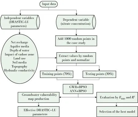
Fig.1 Flowchart showing the methodology used in this study

2.2 DRASTIC-LU model

DRASTIC model has been used to evaluate the capability of groundwater relative contamination vulnerability, using hydrogeological parameters. This model has been constituted from the combination of seven measurable hydrogeological parameters, which are effective on the transfer of contaminants into groundwater, and comprising the depth to water, net recharge, impact of vadose zone, soil media, aquifer media, hydraulic conductivity and topography. At the present study, the land use layer has been added to enhance the accuracy of the model as mentioned earlier.

The distance between the land surface and the water table is called depth to water. In other words, this parameter indicates the depth that a contaminant must pass through to reach groundwater, m[14]. Net recharge is the amount of water that penetrates from the ground surface and reaches into a water table, mm/a[15]. Furthermore, through the increase of net recharge value in a region, the contamination potential of groundwater will rise in that region. The impact of vadose zone comprises the zone between the water table and the unsaturated soil environment[16]. This zone is unsaturated or saturated discontinuously and controls the contaminant passing and its dilution. The soil media is the area above the non-saturated zone and approaches the zone where plant roots penetrate in, or the activity of microorganisms exists[15]. The aquifer media is associated with the component characteristics of the saturated zone, such as the porosity rate, particle types and size[17]. The capability of the hydrogeological characteristics of the aquifer in water transferring and associated contaminants is called hydraulic conductivity[16]. This parameter controls the transport and distribution of contaminants from the injection point inside the saturated zone[15]. The further the hydraulic conductivity is the more will be the possibility of contaminants flowing in the aquifer, so the vulnerability will be more. The topography parameter is the slope of the land surface. The land surface slope affects the movement and penetration of contaminants[17-18]. The less the land slope is, the more will be the contact of a contaminant with the land surface, and subsequently, the more likely will be its penetration into the land. Hence through the decrease of land surface slope, the possibility of aquifer vulnerability increases[16]. Population growth, agricultural, industrial and urban activities and thereupon increasing the land-use change and the usage of groundwater resources, not only has diminished but also has degraded the quality of these valuable resources[19]. In this study, land use as an extension parameter to DRASTIC model has been considered. Actually, due to the increased amount of agricultural and industrial activities in the research case study, it seems that land use has an essential impact on water resource pollutions. Then, this parameter has been integrated into the DRASTIC model.

2.3 Artificial neural network

Artificial neural networks are one of the computational methods inspired by the neural system of the human brain. One of the remarkable characteristics of this type of network is their ability to learn and the ability to generalize this learning, and because of this feature, they make it possible to learn to understand patterns[20]. The most important advantage of artificial neural networks over regression methods for predicting and modeling a pattern is that there is no need for an initial model in linking input and output data[21]. Based on the intrinsic relationships between data, a linear or nonlinear model is established between independent and dependent variables.

In this study, a multilayer perceptron neural network has been used to model groundwater vulnerability. This type of neural network consists of a set of neurons arranged in different layers in a row. The law of multilayer perceptron learning is called the error propagation rule, which is used to estimate unknown network parameters. The multilayer perceptron works in such a way that a pattern is supplied to the network and its output is calculated. Actual output values and desired output cause the network coefficients to change; in such a way that a more accurate output is obtained in later stages. To succeed in network training, its output must be gradually brought closer to the desired output and the error rate must be reduced. The design ANN used in this study is illustrated in Fig.2.

Fig.2 ANN architecture applied in this study[21]

2.4 Geographically Weighted Regression

According to spatial autocorrelation and spatial non-stationarity properties for spatial data, it is less possible to use basic global regressions such as ordinary least square[22]. In this method, the spatial dependencies between the events are considered as weight matrices, and due to the heterogeneity of the environmental factors and the existence of local variation, regression coefficients of the GWR model for observation are measured locally[23-24]. The GWR model is calculated as equation (1)[24]:

(1)

Whereyiis the dependent variable (nitrate concentration);xjis the independent variables (DRASTIC-LU parameters);nis the total random points;εiis the residual GWR model; (ui,vi) denotes the coordinates of the ith point in space andβj(ui,vi) is the regression coefficient for coordinates of the ith point. To calculate the spatial weight matrix, it is necessary to specify the desired kernel function. According to previous research, this study used two kernels including exponential and bi-square these two kernels which are calculated as equation (2) and equation (3), respectively[24-25]:

(2)

(3)

(4)

(5)

Whereβijis the regression coefficient for the factorjin the observationi;βjis the mean regression coefficient of factorjin the total observations andnis the total observations.

To evaluate the ANN and GWR models output the coefficient of determination (R2) is usually used to measure the goodness of fit and theERMSvalue measure the residuals distribution of the observation, which are obtained based on equation (6) and equation (7)[24]

(6)

(7)

Wherenis the total observations;yiis the value for observationi;iis the predicted value for observationiandis the mean value for total observations.

2.5 Binary particle swarm optimization

The particle swarm optimization (PSO) algorithm is an optimization algorithm that makes it less likely to be captured at a local minimum and can search uncertain and complex areas based on probabilistic rules[26]. Also in this algorithm, the solution of the proposed path is not dependent on the initial population and starting from each point in the search space, the solution converges to the optimal solution[26]. After a while, Kennedy and Eberhart[27]introduced the binary PSO algorithm, which, unlike the continuous version of it, is limited to having zero and one (binary) variables and the velocity value can change a particle from zero to one. According to the purpose of this study, the BPSO algorithm has been used. In this algorithm, equation (8)-(10) are used to update the velocity and position of each particle[27]:

Vi(t+1)=wVi(t)+c1r1(pb-Xi(t))+
c2r2(gb-Xi(t))

(8)

Xi(t+1)=Xi(t)+Vi(t+1)

(9)

(10)

WhereVi(t) is the velocity of the particlei;Xi(t) is the position of the particlei;Vi(t+1) is the velocity of the particleiin the next position;Xi(t+1) is the position of the particleiin the next position;pbis the best position of the experience for the particlei;gbis the best position experienced in all particles;c1is the personal learning coefficient;c2is the collective learning coefficient;wis the inertia weight andr1,r1andρare random numbers in the range [0.1]. In this study the steps of the BPSO algorithm (in combination with the ANN and GWR models) are as follows which showed in Fig.3:

Fig.3 Calculation steps of the recommended models

Step1Give the initial value to a population of particles with random positions and velocities.

Step2Training ANN and GWR models and calculating the fitness function (R2) of each particle in this population.

Step3Stop the BPSO algorithm if it reaches the stop criterion (100 iterations), otherwise go to step 4. If the algorithm reaches the condition of stopping, then the selected DRASTIC-LU parameters are the same effective parameters that are prepared with the help of effective parameters of the groundwater vulnerability map.

Step4Determine the pbest and gbest for particles.

Step5Calculate the velocity of each particle and move to the next position based on the relations (go to step 2).

3 Results and Discussion

3.1 Define dependent and independent variables

According to Table 1, in this study, the DRASTIC-LU parameters are considered as independent variables. These parameters, in the order mentioned, form the particle dimension of the BPSO algorithm.

Table 1 Independent variables in this study

Fig.4 illustrates the DRASTIC-LU parameters of the case study. Depth of water has been obtained through 15 piezometers installed in the aquifer in a one-year period from October 2016 to September 2017. In this study, in order to obtain net recharge, the zoning method of changes in aquifer groundwater volume with the help of water level data in the observation wells has been used. Aquifer media and impact of vadose zone were achieved through a log of 19 observation and operation wells in the region through the Regional Water Organization of Southern Khorasan Province. The topography of area has been obtained using a digital elevation model map with a spatial resolution of 15 meters. Hydraulic conductivity has been calculated from the pumping experiment data performed by the Regional Water Organization of South Khorasan Province. For soil type, remote sensing and map data prepared by Agriculture Organization of Southern Khorasan Province were used. Finally, land use was based on Landsat 8 satellite imagery in the Google Earth Engine environment captured in 2017. For the production of DRASTIC-LU maps, a kriging interpolation has been used since this method has the minimum error[13].

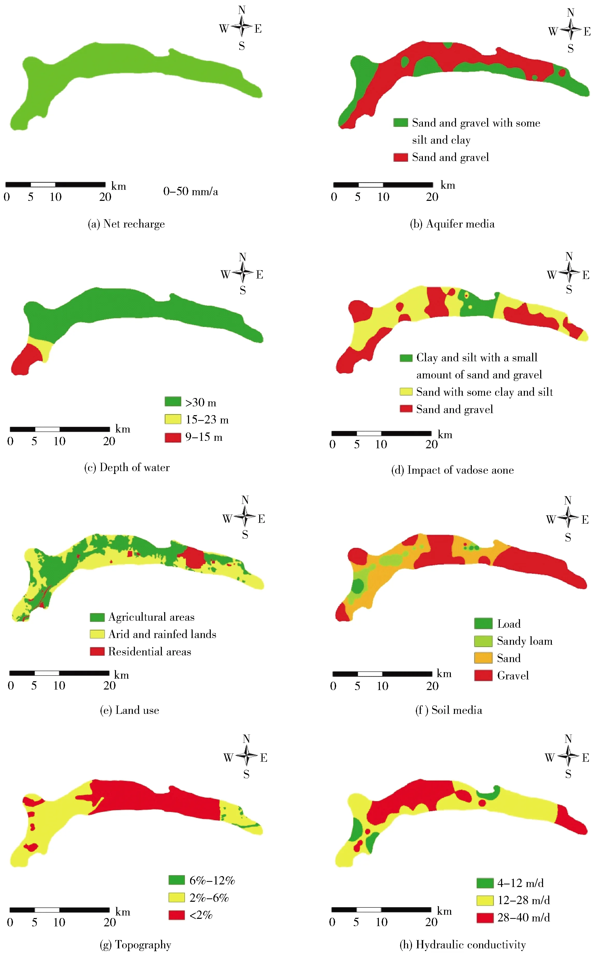
Fig.4 Maps of DRASTIC-LU parameters

In this experiment, the nitrate contents of 21 wells located in Birjand plain aquifer based on the data from the water quality lab of the Water and wastewater department of Birjand city have been used. The applied data is an average of nitrate concentration during five years from 2014-2019. To show the nitrate concentrations all over the Birjand aquifer (10-6, unit); a kriging interpolation has been used (Fig.5(a)).

Fig.5 Map of dependent variable based on observation wells and random points

According to Fig.5(b), after calculating the DRASTIC-LU parameters as independent variables and nitrate concentration as dependent variable, 1 000 points created in the study area by a random sampling method to extract values and use in the GWR-BPSO model[28]. Then the values of all available information parameters (independent and dependent variables) for these points were calculated (in a normalized way). The correlation between the DRASTIC-LU parameters from equation (11) was examined[29]:

(11)

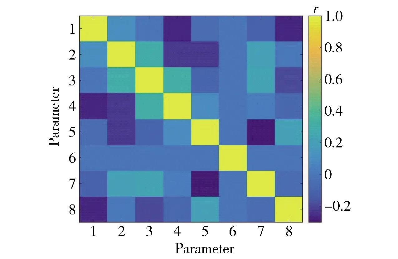
1-8 shown as Table 1. Fig.6 Correlation matrix between DRASTIC-LU parameters

3.2 Implement data-driven models

For the implementation of the ANN and GWR models, 70% of the total data was used for training and 30% of the total data was used for testing, and all data were normalized before entering the algorithms. Based on previous research and trial and error method, a ratio of 70∶30 was selected[30]. In article this ratio gives the best performance result. Due to the fact that one of the most important parameters for evaluating the GWR model (model compatibility with data) is the coefficient of determination parameter (R2), therefore, the BPSO algorithm fitness function has been selected to minimize the value of 1-R2[24]. The optimal values of the initial parameters of the BPSO algorithm were selected based on the experiments obtained from different iterations and through trial and error according to Table 2. The condition for stopping to simplify the implementation process is the number of specific executions.

Table 2 Set parameters in the BPSO algorithm

Fig.7 shows the swarm structure of the BPSO algorithm in this study, which the DRASTIC-LU parameters mentioned in Table 1 form the particle dimension of the BPSO algorithm.

Fig.7 Swarm structure of the BPSO algorithm

Due to the random nature of the BPSO algorithm and based on previous research, this algorithm with the desired number of iterations was repeated 10 executions and the best of these 10 executions was considered as the final output[31]. According to Fig.8(a), by performing the combination of the ANN model and the BPSO algorithm, the best value of fitness function (1-R2) was obtained 0.106 0 (the best of 10 executions). Also, according to Fig.8(b) for the ANN model, 5 parameters of aquifer media, land use, soil media, topography and hydraulic conductivity were determined as effective DRASTIC-LU parameters in predicting nitrate concentration. In fact, Fig.8(b) shows the best particle in terms of fitness function (R2) among all particles (30 particles) in the 100th iteration of the BPSO algorithm.

Fig.8 Results of ANN+BPSO model

Then, the GWR model with two exponential and bi-square kernels and BPSO algorithm was combined to determine the effective DRASTIC-LU parameters in predicting nitrate concentration. To implement the GWR model, the coordinates of the random points were used as inputs in its weight matrix. According to Fig.9, the best value of fitness function (1-R2) for combination the GWR model with two exponential and bi-square kernels and the BPSO algorithm, was obtained 0.074 5 and 0.006 5 (the best of 10 executions), respectively. Also, according to Fig.10 for the GWR model with the exponential kernel, 6 parameters of aquifer media, depth of water, impact of vadose zone, land use, soil media and hydraulic conductivity and for the bi-square kernel, 7 parameters of aquifer media, depth of water, impact of vadose zone, land use, soil media, topography and hydraulic conductivity were determined as an effective DRASTIC-LU parameters in predicting nitrate concentration.

Fig.9 The best value of fitness function by combining of GWR model and BPSO algorithm

Fig.10 Effective DRASTIC-LU parameters in predicting nitrate concentration by combining of GWR model and BPSO algorithm

In Fig.11, the values ofR2and RMSE for the ANN and GWR models are shown. Accordingly, the bi-square kernel has higher accuracy in predicting nitrate concentration based on the DRASTIC-LU parameters.

Fig.11 Comparison of ANN and GWR models in terms of R2 and RMSE

According to Fig.12, the maps of predicted nitrate concentration (based on the DRASTIC-LU parameters) by combining ANN and GWR models and BPSO algorithm showed in the range [0,1]. The estimated nitrate concentration is classified into five output classes according to the equal interval classification method which is shown qualitatively from very low nitrate concentration to very high nitrate concentration. According to the results obtained fromR2value (goodness of fit) and the RMSE value (residuals distribution of the observation and accuracy of model), the combination of GWR model with bi-square kernel and BPSO algorithm has a higher ability to estimate nitrate concentration (groundwater vulnerability), which showed in Fig.12(c).

Fig.12 Map of estimated nitrate concentration

As mentioned, since the regression coefficients are different for each location in the GWR model,local variation and spatial non-stationarity of the regression coefficients can be obtained by the standard deviation function. Therefore, for the GWR method with the two kernels mentioned, the most and least variation between the DRASTIC-LU parameters and groundwater vulnerability with displacement have been investigated. Fig.13 shows the standard deviation of regression coefficients GWR model (with two exponential and bi-square kernels) for calculating the rate of local variation and spatial non-stationarity.

Fig.13 Standard deviation of regression coefficients GWR model with exponential and bi-square kernels

According to Fig.13, for the GWR model with the exponential kernel, the relationship between impact of vadose zone and groundwater vulnerability (nitrate concentration) with displacement has the most variation and the relationship between land use parameter and groundwater vulnerability (nitrate concentration) has the least variation. Also, in the GWR model with the bi-square kernel, the relationship between impact of vadose zone parameter and groundwater vulnerability (nitrate concentration) with displacement has the most variation and the relationship between soil mediaparameter and groundwater vulnerability (nitrate concentration) has the least variation. Finally, global Moran’s index was used to determine the spatial autocorrelation of GWR model residuals, which is calculated from equation (12)[32]:

(12)

Table 3 Values of Moran’s index for GWR model residuals with two exponential and bi-square kernels

4 Conclusions

1) To achieve the main purpose of this study, the spatial and non-spatial data-driven methods including GWR and ANN model were used to predict the nitrate concentration based on the DRASTIC-LU parameters. The results showed that the GWR model used, taking into account the characteristics of spatial autocorrelation and spatial non-stationarity, has higher accuracy in predicting nitrate concentration based on the DRASTIC-LU parameters.

2) In this study, the binary particle swarm optimization algorithm was used in combination with the ANN and GWR models, which showed that the DRASTIC-LU parameters have a significant effect on predicting nitrate concentration in the study area. The important point is that the mentioned method is not limited to this case study and can be used to predict the nitrate concentration in various types of regions.

3) For future works, we propose a more extended statistical period and, if possible, more sampling wells can help building and evaluating the model better. Also we suggest using other evolutionary methods such as genetic algorithm, ant bee colony algorithm, etc. Since the improvement of the DRASTIC model with land use parameter has led to better results in the semi-arid region studied, further improvements of the model in combination with other indices are suggested.