On a tilted Liouville-master equation of open quantum systems

Fei Liu

School of Physics,Beihang University,Beijing 100191,China

Abstract A tilted Liouville-master equation in Hilbert space is presented for Markovian open quantum systems.We demonstrate that it is the unraveling of the tilted quantum master equation.The latter is widely used in the analysis and calculations of stochastic thermodynamic quantities in quantum stochastic thermodynamics.

Keywords: quantum stochastic thermodynamic,tilted quantum master equation,quantum trajectories,Feynman–Kac formula,stochastic heat,Liouville-master equation

1.Introduction

In the past two decades,stochastic thermodynamics for open quantum systems has attracted considerable theoretical interest[1–4].One of the major issues is the statistics of random thermodynamic quantities such as heat,work,entropy production,and efficiency [5–33].The tilted or generalized quantum master equation(TQME)is a useful approach for the study of these problems [1].For instance,the fluctuation theorems of steady-states can be demonstrated according to the symmetries implied in the maximal eigenvalue of the equation[1,21,22,33].To study the concrete probability distributions of the random thermodynamic variables,we can numerically or analytically solve the equation to obtain characteristic functions or moment generating functions [21–23,26,28,29,34]; the distributions and functions are mathematically equivalent.

TQME was developed by Esposito et al [1] in their investigation of the fluctuation theorems of open quantum systems.Their derivation is based on the celebrated twoenergy measurement scheme [5] and the whole procedure is similar to the derivation of the quantum master equation[35–37].Indeed,these two equations appear to be almost the same in form;the only difference is an exponential term in the front of the jump terms therein.Although TQME is established in stochastic thermodynamics,an analogous equation was presented by Mollow in 1975 in a seminal paper about photon emissions of quantum systems with discrete energy levels [38].Importantly,the notion of quantum jumps was proposed in this paper [39,40].To determine the photonnumber distributions in the many modes of fluorescence,Mollow developed a hierarchy of equations.Garrahan and Lesanovsky argued that these equations are equivalent to TQME [11].This result inspired us to re-derive TQME from the perspective of quantum jumps [4,26].Different from the method of Esposito et al [1],our method is based on the unraveling of the quantum master equation into quantum jump trajectories [41],and Dyson expansion is used[26,42].

Although TQME is widely adopted in the literature,several open questions still remain.Quantum jump trajectories,or trajectories for short,are composed of alternating deterministic pieces and random jumps of wave functions of individual quantum systems.They are a type of stochastic process called the piecewise deterministic process (PDP) [43].Hence,in Hilbert space,there exists a Liouville-master equation that governs the dynamics of the probability distribution of the random wave functions.Moreover,this equation exactly yields the quantum master equation for the reduced density matrix[44–47].This naturally raises the following questions: Is there a tilted Liouville-master equation in the Hilbert space?What is the relationship between the equation and the Liouville-master equation?Does it yield TQME?We also list these questions in figure 1.The aim of this paper is to present definite answers to these questions.

The remainder of this paper is organized as follows: In section 2,the Markovian quantum master equation and its unraveling of trajectories are briefly reviewed.In section 3,by defining two functionals,we rewrite the probability distribution functional of the trajectory in a new form.In section 4,a Feynman–Kac formula in the Hilbert space is derived.Based on these two results,in section 5,we derive the tilted Liouville-master equation and demonstrate that it is indeed the unraveling of TQME.section 6 concludes the paper.

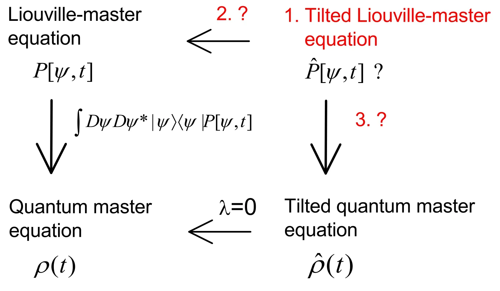
Figure 1.Three questions of interest addressed in this paper:1.Is there a tilted Liouville-master equation in the Hilbert space?2.What is the relationship between it and the Liouville-master equation? 3.Does the equation yield the conventional TQME?

2.Unraveling of Markovian quantum master equation

We start with the Markovian quantum master equation.Because our aim is to prepare the essential equations and notations,the description is brief; a detailed explanation can be found in the standard textbooks,e.g.[41].Letρ(t) be the reduced density matrix of an open quantum system.Under appropriate assumptions and conditions,the ensemble dynamics of the system is described by the Markovian quantum master equation [48–50]

where the Planck constantħis set to 1,H denotes the Hamiltonian of the quantum system,Aαis the Lindblad operator,and non-negative rα,α=1,… ,Mrepresent the correlation functions of the environments surrounding the system.Remarkably,this general equation is also equal to an ensemble average of the density matrices of the individual stochastic quantum systems [44–47]:

Here,Dψ Dψ* is the Hilbert space volume element,andP[ψ,t] is the probability distribution functional of the random wave function ψ at time t.The latter satisfies the Liouville-master equation [37,47]:

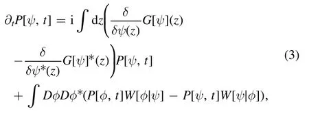
where δ[] denotes the Dirac functional,kα[φ] =rα‖Aαφ‖2is the rate of jump of the wave function from φ to the targetψα=Aαφ‖Aαφ‖,and the precise definition of the latter is given in equation (7) below.Equation (3) is called the unraveling of the quantum master equation (1).

The stochastic process underlying equation (3) is the PDP in the Hilbert space [37].The evolutions or trajectories of the individual quantum systems are composed of deterministic pieces and random jumps [37]: the former are the solutions of the nonlinear Schrödinger equation

while the latter are the instantaneous jumps of wave functions given by

α=1,… ,M,and the rates of the jumps are nothing butkα[ψ(τ)].The target wave functionsψαin equation(7)appear to depend on the concrete wave functionsψ(τ) at the jumping times.However,in the cases of physical interest,they are uniquely specified by the Lindblad operators Aα[37].In this paper,we consider only such cases.

3.Probability distribution functional of trajectory

Let us denote the trajectories of the individual quantum systems asΨt,where t denotes the duration of the quantum nonequilibrium process.We denote the jumps along a trajectory byαi∈ {1,… ,M},and i represents the time tiin which the ith jump occurs,wherei=0,1,… ,N,and N is the total number of jumps.Then,the probability distribution functional of monitoring a trajectoryΨtis simply [37]

where we use the subscript 0 on the left-hand side to denote the initial wave function of the quantum system being in a target wave functionψα0,andψ)is the wave function of the system immediately prior to the jumping time ti.The total rate of jumps is

We emphasize that in the time interval between tiandti+1,ψ(s)follows the solution of equation (6); the initial condition is specified by the target wave function after the last jump,that isψ(s=)=ψαiandis the time immediately after the jump.The exponential decay function in equation (8) implies that during the successive evolutions,the quantum system has a probability of jumping from the current state to the potential target wave functions.This is the physical consequence arising from irreversible dissipations induced by environments or from continuous measurements on the individual quantum systems[37,51,52].

The probability distribution functional of the trajectory (8) has an alternative form:

where we define two functionals

andδα,α iis the Kronecker delta symbol.It is not difficult to see that equation (11) represents the fraction of time of the quantum system occupying the wave function φ in the duration t,while equation (12) is the empirical rate of jumping from the special φ to the special targetψα.At long time limits,we expect that these functionals reduce to the probability distribution of wave functions and flows of the steady-state of the quantum ensemble,respectively.Equation(10)can be used to obtain the rate functional of the level 2.5 large deviations of open quantum systems [32,53].We do not pursue this issue in this paper.

To close this section,we introduce notation for formally expressing the ensemble average of an arbitrary functionalO[Ψt]of trajectories:

whereP[ψα0]represents the initial probability distribution functional and the summations are over all possible trajectories and initial target wave functions.Although equation (13) is not rigorous,it is adequate to support our below discussions.

4.A Feynman–Kac formula

In this section,we present a Feynman–Kac formula for the PDPs in the Hilbert space.The basis of our discussion is the intuitive picture of the trajectories and simple relations among the probabilities in equations (6) and (7).Consider a timedependent integral

We assumeu(t) to be a continuous real function of time t.Obviously,the integral is also a functional of the trajectories.

Our aim is to calculate the probability distributionp(u,t)of the random variableu(t) .To this end,we need several intermediate quantities and equations.First,we defineP[ψ,u,t]as the probability distribution functional of finding the individual quantum systems with wave function ψ and the integral (14) equal to u at time t.We havep(u,t) =∫Dψ Dψ*P[ψ,u,t].Moreover,we define again another functionalP[ψ,u,t;ψα,v,τ]: it represents the joint probability distribution functional when the wave function of the quantum system and the integral at time t are ψ and u,respectively,the successive time of evolution is τ,the target wave function and the integral at the time of last jump are equal toψαand v,respectively.These two distribution functionals are related by

where the integration ∫dvis over the whole space of the random variableu(t) .

Let h be a small time interval.We can write a probability formula about the detailed probability distribution functional as follows:

The reason for this is that if the quantum system starts with the target stateψαwith a value v of the integral (14),and successively evolvesτ+hat timet+h,the system must also evolve τ at time t,and no jumps occur during the interval h.We note that both the Dirac functional δ[]and function δ()therein are the consequences of the deterministic equation(6).We expand both sides of equation (16) in terms of h until its first order:

Letting h tend to zero and using the properties of the Dirac delta function and functional,we obtain

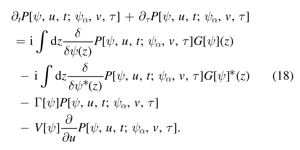
On the other hand,P[ψ,u,t;ψα,v,τ=0] is also equal to the probability distribution in which other wave functions jump toψαat time t,and these functions may start with different target wave functions with various successive times of evolution.Hence,we can reformulate it as

Equation(19)appears to be somewhat lengthy.Nevertheless,the mean of probability is clear.According to equation (15),by integrating and summing equation (18) over τ and α,respectively,we obtain a differential equation for the probability distribution functionalP[ψ,u,t]as follows:

We are close to the Feynman–Kac formula.Defining Laplace transform ofP[ψ,u,t]with respect to the variable u,

and using equation (20),we derive an equation for the new functional:

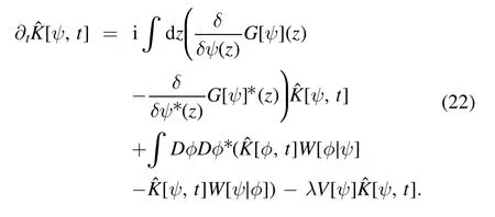
Because the Laplace transform Φ(λ)of the probability distribution functionp(u,t) for the integral (14) is simply related to[ψ,t] as

if the latter is solved by equation (22),we can calculatep(u,t)by performing an inverse Laplace transform of Φ(λ).Finally,becausep(u,t) has an expression of an ensemble average of the trajectories,equation (23) also leads to

We name the collection of equations (22) and (24) as the Feynman–Kac formula of the PDP in the Hilbert space.This is a quantum counterpart of the classical version in the space of classical states [43].

5.Tilted Liouville-master equation

In quantum stochastic thermodynamics,the statistics of heat are of great interest and play a central role [1].According to the interpretation of quantum thermodynamics,the random jumps of wave functions along quantum trajectories indicate that discrete amounts of heat(the energy quanta)are released to or absorbed from the environment surrounding the quantum systems[2,4–6,15,16,26,33,54].We write the heat in a general form:

whereωαiare some energy constants that are determined by the target wave functions at time points tiof the jumps,e.g.the Bohr frequencies [26,37].The whole term in the circle brackets of equation (25) is similar to equation (12).It is indeed an integration of the latter,that is,∫Dφ Dφ*Fφ,α[ Ψt] .

Now,we can construct a differential equation for the heat.Analogous to previous cases,we focus on its Laplace transform (or the moment generating function) rather than distribution: Ξ(λ) = 〈e xp( -λQ)〉,and the right-hand side of the equation is

Equation(26)inspires us to define an auxiliary open quantum system as follows: its nonlinear Schrödinger equation is the same as equation (6),but the rates of the jumps of wave functions are modified to

In the remainder of this paper,we always denote quantities in the auxiliary open quantum system with a prime symbol unless stated otherwise.With these notations,we can rewrite the Laplace transform of the heat as

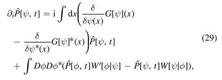
We note that the probability distribution functionalP [ Ψt]of monitoring the trajectoryΨtis the same as equation(8)except that the rates therein are replaced by equation (27).So is the total rate Γ′[ψ] ; see equation (9).Defining the integrand of equation (28) asPˆ[ψ,t] and using the Feynman–Kac formula (22) and (24),we immediately obtain

where

We name equation (29) the tilted Liouville-master equation,which is the central result of this paper.If λ is zero,the equation yields the Liouville-master equation (3).Hence,we have definitely answered the first two questions in figure 1.

5.1.Tilted quantum master equation

Here,we demonstrate that equation (29) can yield the tilted quantum master equation [1],i.e.the third question of this paper.The procedure is very similar to that of the Liouvillemaster equation and quantum master equation[44–47].Let us consider an operator(t) that is defined as

in the position representation.Taking the time derivatives of its both sides and substituting equation (29),we have

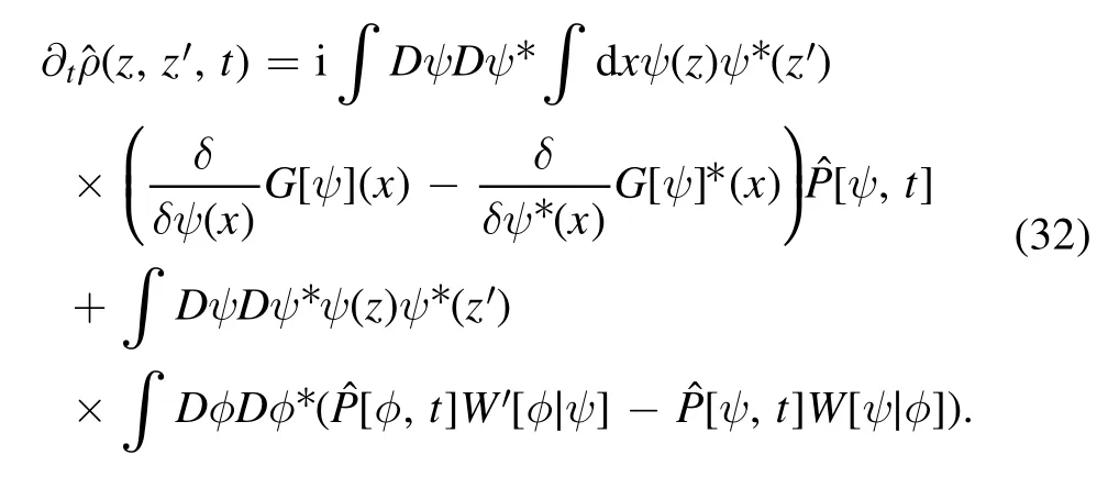
There are four terms on the right-hand side of equation (32).The first term is equal to

The first equation of equation (33) uses the functional integration by parts.Because of the properties=δ(z-x)and=0,we arrive at the second equation.The third equation therein is a consequence of inserting equation (4).Performing similar calculations,the second term of equation (32) is

By inserting equation (30),we can rewrite the third term as

The fourth term is relatively simple:

Equations (33)–(36) appears tedious.However,when we substitute them into the right-hand side of equation (32),we find that this differential equation leads to a concise form for the operator(t) :

Accordingly,an alternative expression for the Laplace transform of the heat is obtained: Ξ(λ) =Tr[ρˆ(t)].Equation(37)is nothing but TQME [1].Analogous to the relationship between equations (1) and (3),we name equation (29) the unraveling of equation (37) in Hilbert space.Because of the absence of the abstract functional derivatives,the latter is more advantageous for the calculation and analysis of the statistics of random heat (25).

6.Conclusion

We have obtained the tilted Liouville-master equation in the Hilbert space and this equation can yield the tilted quantum master equation of open quantum systems.

Acknowledgments

We appreciate Professor Hong Qian and Dr Carollo for their inspiring discussions.This work was supported by the National Science Foundation of China under Grant No.11174025 and No.11575016.

ORCID iDs