Analytic approximate solutions of diffusion equations arising in oil pollution

Hijz Ahm ,,Tufil A.Khn ,Hüly Durur ,G.M.Ismil ,,Asıf Yokus

a Department of Basic Sciences,University of Engineering and Technology,Peshawar,25000,Pakistan

b Department of Computer Engineering,Faculty of Engineering,Ardahan University,Ardahan,75000,Turkey

c Department of Mathematics,Faculty of Science,Sohag University,Sohag,82524,Egypt

d Department of Actuary,Faculty of Science,Firat University,Elazig,23200,Turkey

e Department of Mathematics,Faculty of Science,Islamic University of Madinah,170,Madinah,Saudi Arabia

Abstract In this article,modified versions of variational iteration algorithms are presented for the numerical simulation of the diffusion of oil pollutions.Three numerical examples are given to demonstrate the applicability and validity of the proposed algorithms.The obtained results are compared with the existing solutions,which reveal that the proposed methods are very effective and can be used for other nonlinear initial value problems arising in science and engineering.

Keywords:Modified variational iteration algorithm-II;Diffusion equation;Allen-Cahn equation;Parabolic equation;MVIA-I.

1.Introduction

Partial differential equations (PDEs) are studied in various fields such as astrophysics,fluid mechanics,solid-state physics,ocean engineering,plasma physics,optical fibre,wave motion,ocean ecology,and metrology and have been studied by many scientists for many years.

Oil pollution is the release of a fluid oil hydrocarbon into the ocean environment because of human activities such as releases of unrefined petroleum from tankers,drilling rigs,offshore platforms as well as piping and may cause serious damage to the marine ecological environment.Therefore,a precise guess of behaviours of these oils is extremely noteworthy to keep the seaside natural environmental system.The zone of oil spreading can be anticipated numerically by the solution of proper equations governing the flow field and the diffusion phenomenon.The most reasonable choice is probably the diffusion equations where the information about the quantity of oil,which reached the ocean outlet can be taken as initial and boundary conditions for modelling of oil diffusion and alteration in the waters.

To describe oil pollution,consider the general nonlinear diffusion equation of the form:

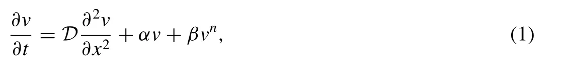
Wherevis concentration,Dis diffusion coefficient,α andβare real constants.Eq.(1) becomes Allen-Cahn equation whenn=3,α=1andβ=−1,which has various applications in quantum mechanics,biology and plasma physics[1].

There are various analytical and numerical methods for the solution of nonlinear equations i.e.the finite difference method [2,3],Modified Kudryashov method [4],Sumudu transform method [5],(1/G＇)-expansion method [6],expansion methods [7,8],finite element method [9],Hirota’s bilinear method [10,11],Decomposition methods [12–15],variational iteration algorithm-I [16–20],function transformation method [21],simple equation method [22],simplified Hirota method [11],variational method [22–24],direct algebraic method [25],modified direct algebraic method [26],Exp-function method [27],Homotopy perturbation method[28–31],parameter expansion method [32],homotopy analysis method [33–35],Fourier pseudospectral method [36],modified auxiliary equation method [36],variational iteration method [37–43],(G＇/G)-expansion method [36],Taylor series method [44]and so on.

The Allen–Cahn (AC) equation appears in various studies,such as numerical solutions of AC equation are obtained by using the finite difference method [2],obtained new exponential prototype structures to the AC model using Bernoulli sub-equation function method [45],studied nonlınear stability of the Implicit-Explicit methods for AC equation [46],Gui and Zhao [47]studied the existence and qualitative properties of travelling wave solutions of the AC equation and so on.

This research paper aims to achieve numerical solutions of the diffusion and Allen–Cahn (AC) equations by using modified versions of variational iteration algorithms,which are the advancements of the variational iteration method proposed by Ji-Huan He [48].The organization of the rest of the paper is as follows;in Section 2,modified versions of variational iteration algorithms are described.In Section 3,some problems are investigated to show the accuracy and applicability of the suggested technique and in the last Section 4,a detailed conclusion is discussed.

2.Modified versions of variational iteration algorithms

Consider the following nonlinear differential equation

Where theL[v(ς)]andN[v(ς)]are linear and nonlinear terms respectively,whilea(ς) is the source term.For Eq.(2) correction function can be written as below:

Which is an iterative scheme for variational iteration algorithm-I,whereλis known as the Lagrange multiplier[49],its values can be obtained by using optimality conditions.whereis a restricted term which in turn gives=0.Thus

This gives an exact solution after some iterations

Summarizing the iterative algorithm for Eq.(1) is,

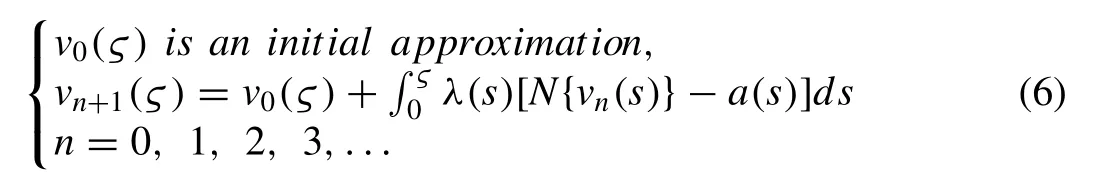
The iterative algorithm (6) is named as variational iteration algorithm-II [50–54]abbreviated as (VIA-II),which is a modified form of Lagrange multiplier technique [49].Recently,this method has been active for offering numerical as well as analytical solutions for a vast range of complications arising in several fields of engineering and physical sciences.

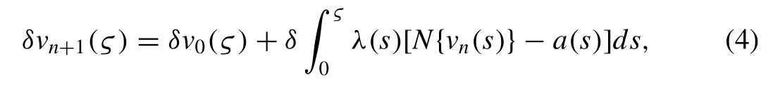
In the wake of presentingh,algorithm (6) takes the structure;

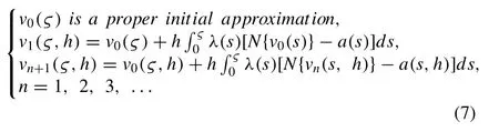
This iterative algorithm is named as MVIA-II.We employ this adapted process for the solution of Allen-Cahn and diffusion equations.

3.Numerical applications

This section is devoted to the numerical implementation of modified versions of the variational iteration algorithms for different types of Allen-Cahn equations and a diffusion equation.Here,the approximate solutions to the diffusion and Allen-Cahn equations are gained easily and smartly with neither use of conversion nor linearization.

3.1. Example 1 (diffusion equation)

First,Consider the diffusion equation [55]

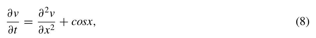
The given conditions are:

The given exact solution is:

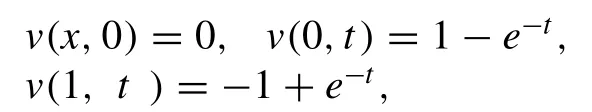
We begin with the construction of the correction function of MVIA-I for Eq.(8) as,

The value ofλ(η) can be found out most quickly by using variational theory.

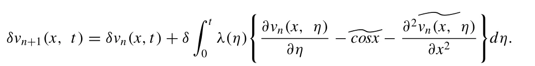
Ignoring the restricted terms

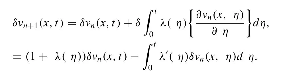
Fig.1.Absolute error graph in space-time graph form for 10th iteration by VIA-I corresponding to the Example 1.

The stationary conditions are:λ＇(η)=0,1 +λ(η)=0,we get a scalar value ofλ(η),which isλ(η)=−1.Using this scalar value ofλ(η) in Eq.(10) gives the following recurrence relation:

Starting the procedure by using an appropriate initial guess for the problem,

other iterations can be obtained by utilizing the recurrence relation (11),

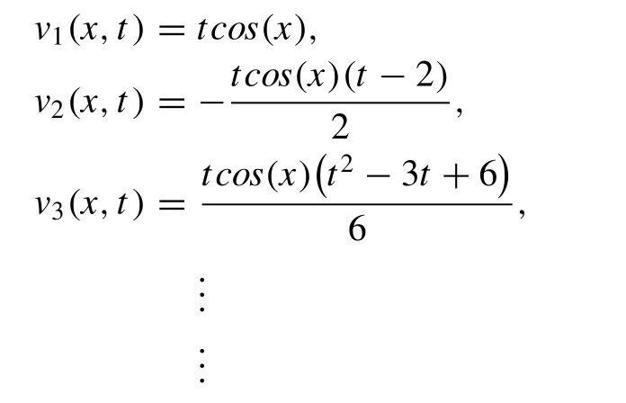
we terminate the procedure atv10(x,t).The absolute error ofv10(x,t) in the domain of solution(x,t)∊[ 0,10 ]× [ 0,5 ]can be seen in Fig.1.

Now,solving the above system of linear diffusion equation by MVIA-I.Using the modified algorithm MVIA-I,the recurrence relation for Eq.(8) can be written as

Starting the procedure by using the appropriate initial guess for the problemv0(x,t)=0,other iterations can be obtained by utilizing the recurrence relation (12),

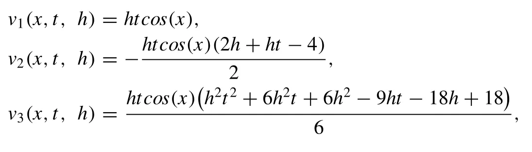
we terminate the procedure atv10(x,t,h).A residual function for obtaining an optimal value ofhcan be defined as

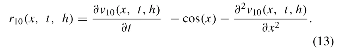
The square of residual function for 10thiteration with respect tohfor(x,t)∊[ 0,10 ]×[ 0,5 ]is

The residual function (13) can be used to approximatee10(h) and the proper value ofhcan be found out by makinge10(h) minimum.The optimal value ofhis determined to be 0.85683707022111,whene10(h) is minimized.We may get extra accurateness by increasing the numeral of iterations.Putting the value ofhinv10(x,t,h) in the domain of solution(x,t)∊[ 0,10 ]× [ 0,5 ],the absolute error can be seen in Fig.2.

Comparing Figs.1 and 2,we confirmed that the modified algorithm:MVIA-I gives more accurate results than the classical algorithm.Comparison of absolute errors of VIA-I and MVIA-I for different values of parameters is given in Table1.

3.2. Example 2 (Allen-Cahn equation)

Consider the AC equation [1]of the form,

with the initial condition:

The exact solution is given by:

Fig.2.Absolute error graph in space-time graph form for 10th iteration by MVIA-I corresponding to Example 1.

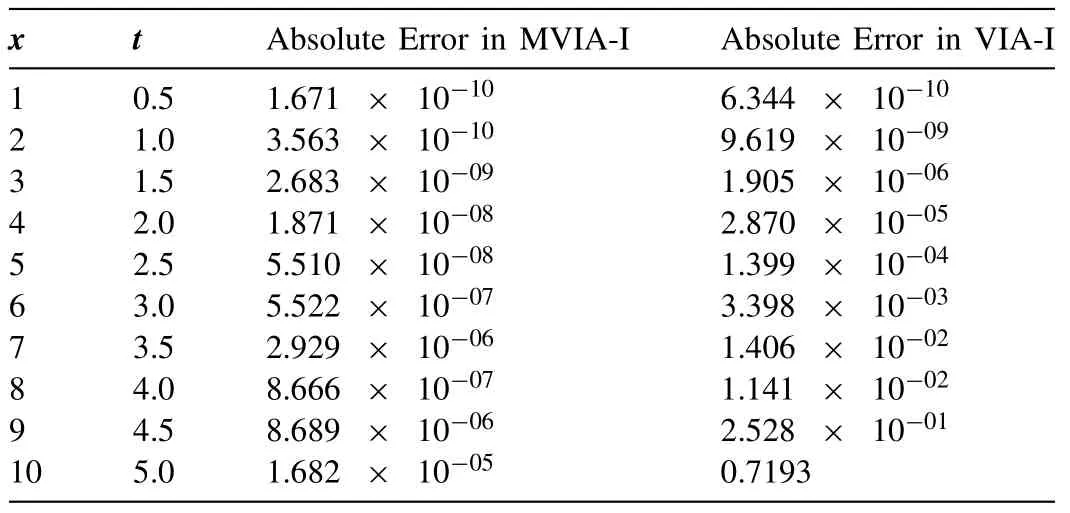
Table1 Comparison of absolute errors for 10th iteration corresponding to Example 1.

To start with,we solve the above system of AC equation by VIA-II.Making the correction function for the Eq.(15) as,

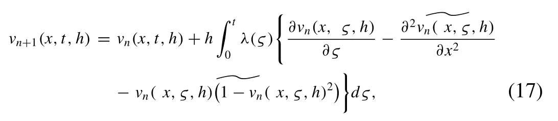
Using the value ofλ(ς),which is -1 obtained by the variational principle [56–58]in Eq.(17),results in the below correction function:

Starting with an initial condition

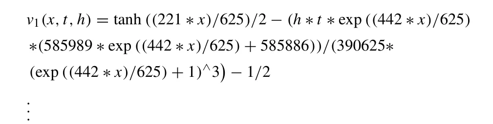
The following different iterations can be obtained with the use of recurrence relation (18),

For finding the optimal value ofhfor the estimated solution,the subsequent residual function is delineated:

The norm 2 of residual function (19) for 3rd-order approximation for(x,t)∊[ 0,30 ]×[ 0,1 ]is

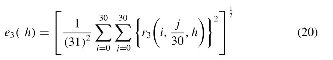
The residual function (19) can be used to approximatee3(h) and the proper value of h can be found out by makinge3(h) minimum.The optimal value ofhis determined to be 0.956746100698240,whene3(h) is minimized.We may get extra accurateness by increasing the numeral of iterations.Utilizing this optimal value ofhinv3(x,t,h) in the domain(x,t)∊[ 0,30 ]× [ 0,1 ],the following results are obtained,which can be seen in Table2,Figs.3 and 4.

3.3. Example 3 (AC Equation)

Consider the AC equation [2]of the following form

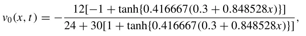
with the initial condition:

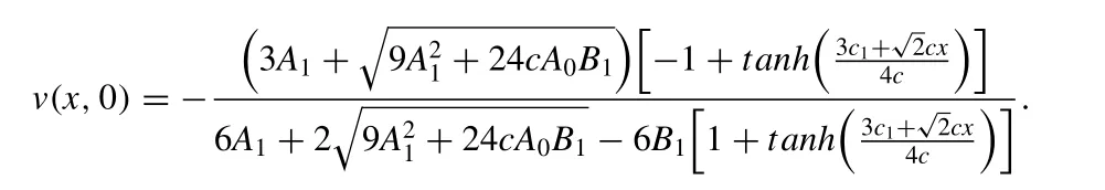
WhereA0=−3,c=0.6,B1=−5,A1=−1,c1=0.1

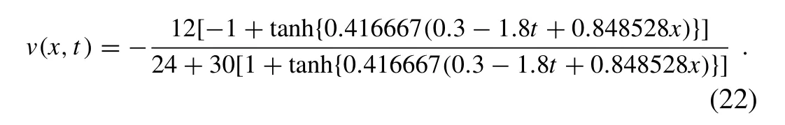
The exact solution of Eq.(21) with the above assumptions:

Fig.3.Behavior of approximate solution (above) and exact Solution (below) corresponding to Example 2.

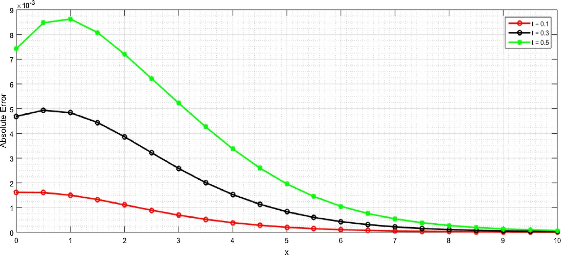
Fig.4.Comparing the curves of absolute errors for different values of t corresponding to Example 2.

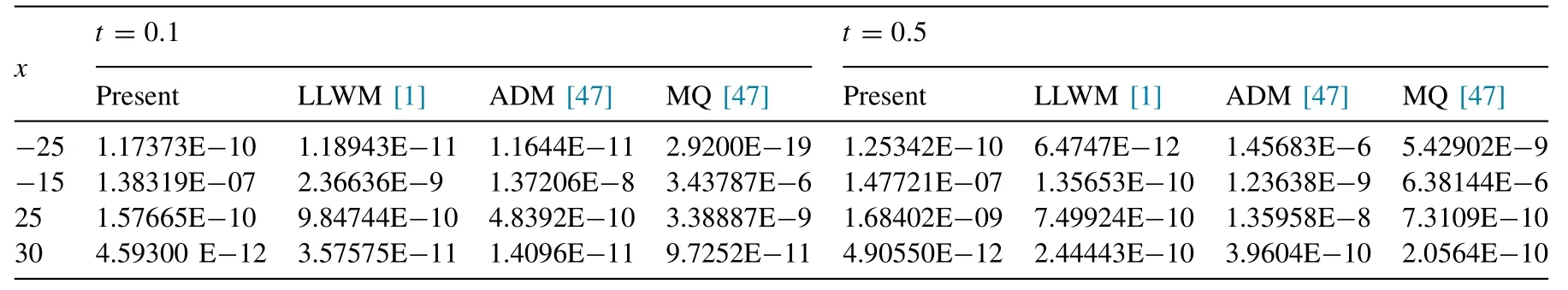
Table2 Comparison of absolute errors for different values of t and x corresponding to Example 2.

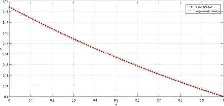
Fig.5.Comparison of exact and approximate solutions for t=0. 01 corresponding to Example 3.

To start with,we solve the above system of AC equation by VIA-II.Making the correction function for the Eq.(21) as,

Using the value ofλ(ς),which is -1 obtained by the variational principle [56–58]in Eq.(23),results in the below correction function:

Starting with an initial condition

The other different iterations can be obtained with the use of recurrence relation (24),For finding optimal value ofhfor estimated solution,the subsequent residual function is delineated:

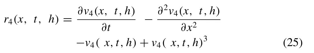
The norm 2 of residual function (25) for 4th-order approximation for(x,t)∊[ 0,1 ]×[ 0,1 ]is

The residual function (25) can be used to approximatee4(h) and the proper value ofhcan be found out by makinge4(h) minimum.The optimal value ofhis determined to be 1.00971373400743,whene4(h) is minimized.We may get extra accurateness by increasing the numeral of iterations.Utilizing this optimal value ofhinv4(x,t,h) in the domain(x,t)∊[ 0,1 ]× [ 0,1 ],more accurate results are obtained,which are reported in Table3,while comparison of exact and approximate solutions can be seen in Fig.5

The numerical results for diffusion equation are reported in Table1,while for AC equations are reported in Table2 and Table3.To prove the effectiveness of the planned techniques,absolute errors are reported along with the results of other methods;finite difference method [2],Adomian’s decomposition [47],multiquadric quasi-interpolation methods [47]andLLWM [1].In comparison with other techniques results,one can ensure that the results of modified variational iteration algorithms are more precise.It is cleared from figures that the proposed algorithms can handle the problems accurately and will be applicable in ocean engineering for studying linear and nonlinear water waves.

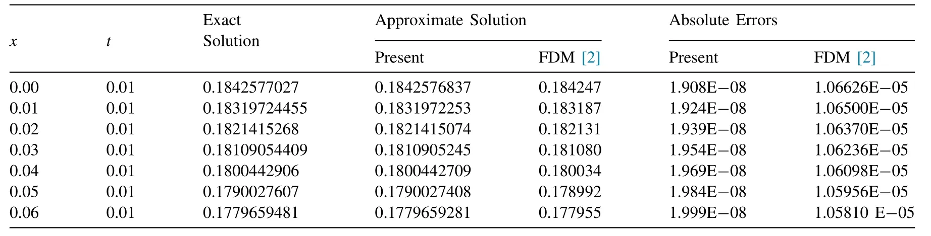
Table3 Comparison of numerical results for different values of t and x for Example 3.

4.Conclusions

In this study,approximate solutions of diffusion equation arising in oil pollution and different types of AC equations are obtained by using two modified algorithms.Based on the results,it has been found that the applied methods will be able to use without using discretization,shape parameter,Adomian polynomials,transformation,linearization or restrictive assumptions and thus are particularly perfect with the expanded and flexible nature of the physical problems and can be easily extended to fractal calculus [59–62]arise in ocean engineering and science.

Declaration of Competing Interest

The authors declare that they have no known competing financial interests or personal relationships that could have appeared to influence the work reported in this paper.