Robust Latent Factor Analysis for Precise Representation of High-Dimensional and Sparse Data
2021-04-13DiWuMemberIEEEandXinLuoSeniorMemberIEEE
Di Wu, Member, IEEE and Xin Luo, Senior Member, IEEE
Abstract—High-dimensional and sparse (HiDS) matrices commonly arise in various industrial applications, e.g.,recommender systems (RSs), social networks, and wireless sensor networks. Since they contain rich information, how to accurately represent them is of great significance. A latent factor (LF) model is one of the most popular and successful ways to address this issue. Current LF models mostly adopt L2-norm-oriented Loss to represent an HiDS matrix, i.e., they sum the errors between observed data and predicted ones with L2-norm. Yet L2-norm is sensitive to outlier data. Unfortunately, outlier data usually exist in such matrices. For example, an HiDS matrix from RSs commonly contains many outlier ratings due to some heedless/malicious users. To address this issue, this work proposes a smooth L1-norm-oriented latent factor (SL-LF) model. Its main idea is to adopt smooth L1-norm rather than L2-norm to form its Loss, making it have both strong robustness and high accuracy in predicting the missing data of an HiDS matrix. Experimental results on eight HiDS matrices generated by industrial applications verify that the proposed SL-LF model not only is robust to the outlier data but also has significantly higher prediction accuracy than state-of-the-art models when they are used to predict the missing data of HiDS matrices.
I. INTRODUCTION
IN this era of information explosion, people are frequently inundated by big data from various industrial applications[1]–[5], e.g., recommender systems (RSs), social networks,and wireless sensor networks. Among these applications,matrices are commonly adopted to represent the relationship between two types of entities. For example, a user-item rating matrix is frequently seen in recommender systems (RSs)[6]–[9], where each row indicates a specific user, each column indicates a specific item (e.g., movie, electronic product, and music), and each entry indicates a user’s preference on an item.
In big data-related applications like Amazon [10], since the relation among numerous entities is unlikely to be fully observed in practice, matrices from these applications are usually high-dimensional and sparse (HiDS) [7], [11]. Yet these HiDS matrices contain rich formation regarding various valuable knowledge, e.g., user’s potential preferences on items in RSs. Hence, how to precisely extract useful information from an HiDS matrix becomes a hot yet thorny issue in industrial applications.
Up to now, various approaches and models are proposed to address this issue [6]–[9]. Among them, a latent factor (LF)model, which originates from matrix factorization techniques[11], [12], is becoming increasingly popular due to its high accuracy and scalability in industrial applications [13], [14].Given an HiDS matrix, an LF model represents it by training two low-dimensional LF matrices based on its observed data only [13], [15]. To model an accurate LF model, how to design its Loss function is very crucial, where Loss denotes the sum of errors between observed data (ground truths) and predicted ones computed by a specific norm on an HiDS matrix [13], [14].
Currently, most LF models adopt L2-norm-oriented Loss[12]–[18] while few ones adopt L1-norm-oriented Loss [19].Fig.1(a) illustrates the differences between L1-norm-oriented and L2-norm-oriented Losses [19]–[21] where Error denotes the errors between predicted results and ground truths: 1) the former is less sensitive to Error than the latter, thereby enhancing the robustness of a resultant model [19], [21], [22],and 2) the latter is smoother than the former when the absolute value of Error is small (less than 1), thereby enhancing the stability of a resultant model [23].
Hence, although an LF model with L2-norm-oriented Loss can achieve a steady and accurate prediction for the missing data of an HiDS matrix space [23], its robustness cannot be guaranteed when such a matrix is mixed with outlier data.Unfortunately, outlier data usually exist in an HiDS matrix.For example, an HiDS matrix from RSs commonly contains many outlier ratings due to some heedless/malicious users(e.g., a user rates an item randomly in the feedback or badmouths a specific item) [24], [25].
On the other hand, although an LF model with L1-normoriented Loss has intrinsic robustness, its solution space for predicting the missing data of an HiDS matrix is multimodal.The reason is that L1-norm-oriented Loss is not smooth when the predicted results and ground truths are close to each other.As a result, an LF model with L1-norm-oriented Loss may be stacked by some “bad” solutions, making it unable to guarantee high prediction accuracy.
From the aforementioned discussions, we see that both L1and L2-norm-oriented Losses are not the best choice for modeling an LF model. Then, do we have an alternative one?This work aims to answer it. Fig.1(b) illustrates the smooth L1-norm-oriented Loss, where we observe that Loss not only is robust to Error but also has a smooth gradient when the absolute value of Error is smaller than 1. Motivated by this observation, we propose a smooth L1-norm-oriented latent factor (SL-LF) model. Its main idea is to adopt smooth L1-norm to form its Loss, making it have both strong robustness and high accuracy in predicting the missing data of an HiDS matrix.
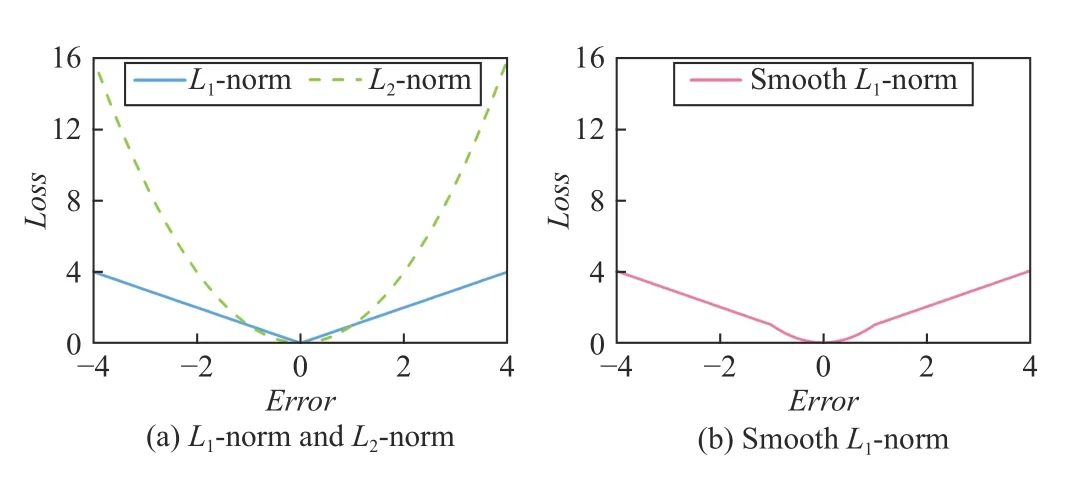
Fig.1. The relationship between Loss and Error with different norms to solve a regression problem.
Main contributions of this work include:
1) Proposing an SL-LF model with strong robustness and high accuracy in predicting the missing data of an HiDS matrix.
2) Performing a suite of theoretical analyses and algorithm designs for the proposed SL-LF model.
3) Conducting extensive empirical studies on eight HiDS matrices generated by industrial applications to evaluate the proposed model and other state-of-the-art ones.
To the author’s best knowledge, this is the first study to employ smooth L1-norm to implement an LF model for predicting the missing data of an HiDS matrix. Experimental results demonstrate that compared with state-of-the-art models, SL-LF achieves significant accuracy gain when predicting missing data of an HiDS matrix. Its computational efficiency is also highly competitive when compared with the most efficient LF models.
The rest of the paper is organized as follows. Section II states preliminaries. Section III presents an SL-LF model.Section IV reveals experimental results. Section V discusses related work. Finally, Section VI concludes this paper.

II. PRELIMINARIES

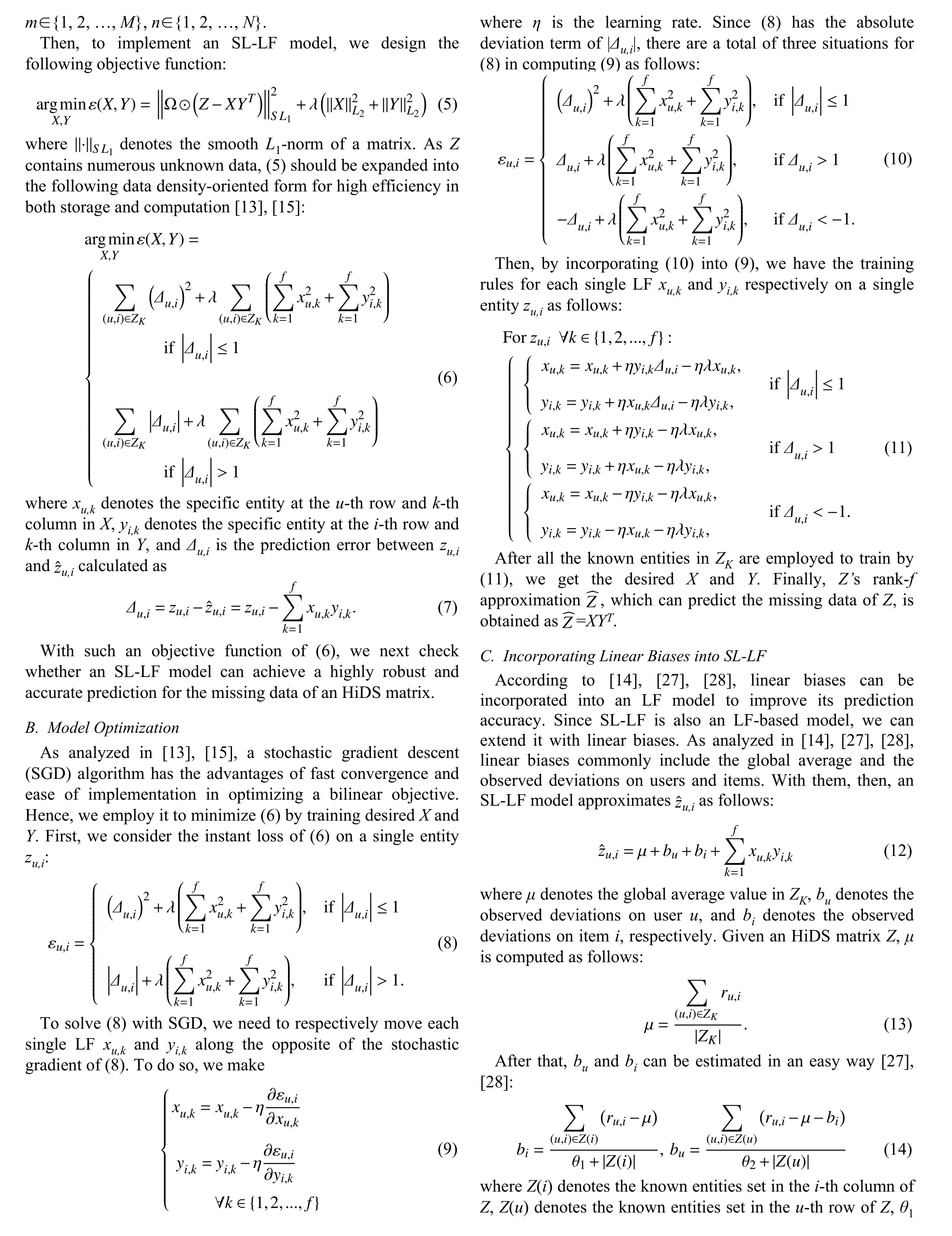

IV. EXPERIMENTS AND RESULTS
A. General Settings
Datasets: Eight benchmark datasets are selected to conduct the experiments. Table I summarizes their properties. They are real HiDS datasets generated by industrial applications and frequently adopted by prior studies [13], [29]. Dating is collected by an online dating website LibimSeTi [30], Douban is collected by Douban.com [13], [29], Eachmovie is collected by the EachMovie system by the DEC Systems Research Center [1], [31], Epinion is collected by Trustlet website [29],Flixter is collected by the Flixter website [32], Jester is collected by the joke-recommender Jester [32], and MovieLens_10M and MovieLens_20M are collected by the MovieLens system [33].

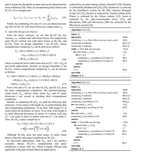
LF¯b Algorithm 1 SLInput: ZK Operation Cost initializing f, λ, η, Nmtr (Max-training-round count) Θ(1)initializing X randomly Θ(|U|×f)initializing Y randomly Θ(|I|×f)while t ≤ Nmtr && not converge ×Nmtr for each entity zu,i in ZK ×|ZK| for k=1 to f ×f computing xu,k according to (7) and (11) Θ(1) computing yi,k according to (7) and (11) Θ(1) end for − end for − t=t+1 Θ(1)end while −Output: X, Y Algorithm 2 SL-LFb Input: ZK Operation Cost initializing f, λ, η, Nmtr (Max-training-round count) Θ(1)initializing X randomly Θ(|U|×f)initializing Y randomly Θ(|I|×f)computing μ according to (13) Θ(|ZK|)for each entity zu,i in ZK ×|ZK| computing bi according to (14) Θ(1)end for −for each entity zu,i in ZK ×|ZK|computing bu according to (14) Θ(1)end for −while t ≤ Nmtr && not converge ×Nmtr for each entity zu,i in ZK ×|ZK| for k=1 to f ×f computing xu,k according to (11) and (15) Θ(1) computing yi,k according to (11) and (15) Θ(1) end for − end for − t=t+1 Θ(1)end while −Output: X, Y
Evaluation Metrics: Missing data prediction is a common but important task in representing an HiDS matrix [34]. To evaluate prediction accuracy, mean absolute error (MAE) and root mean squared error (RMSE) are widely adopted:

where Γ denotes the testing set and |·|absdenotes the absolute value of a given number. Lower MAE and RMSE indicate higher missing data prediction accuracy. Besides, to evaluate the computational efficiency of missing data prediction, we measure CPU running time.
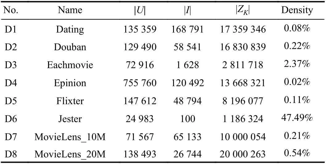
TABLE I PROPERTIES OF ALL THE DATASETS

Experimental Designs: For each dataset, its 80% known data are used as a training dataset and the remaining 20% ones as a testing dataset. Five-fold cross-validations are adopted.All the experiments are run on a PC with 3.4 GHz i7 CPU and 64 GB RAM. In the next experiments, we aim at answering the following research questions:
1) How do the hyper-parameters of an SL-LF model impact its prediction performance?
2) How do the outlier data impact the prediction performance of an SL-LF model?
3) Does the proposed SL-LF model outperform related state-of-the-art models?
B. Hyper-Parameter Sensitivity Tests

1https://pan.baidu.com/s/1o_8sKP0HRluNH1a4IWHW8w, Code: t3sw

Fig.2. The training process of SL-L Fb¯ with different f on D8, where λ =0.01 and η = 0.001.
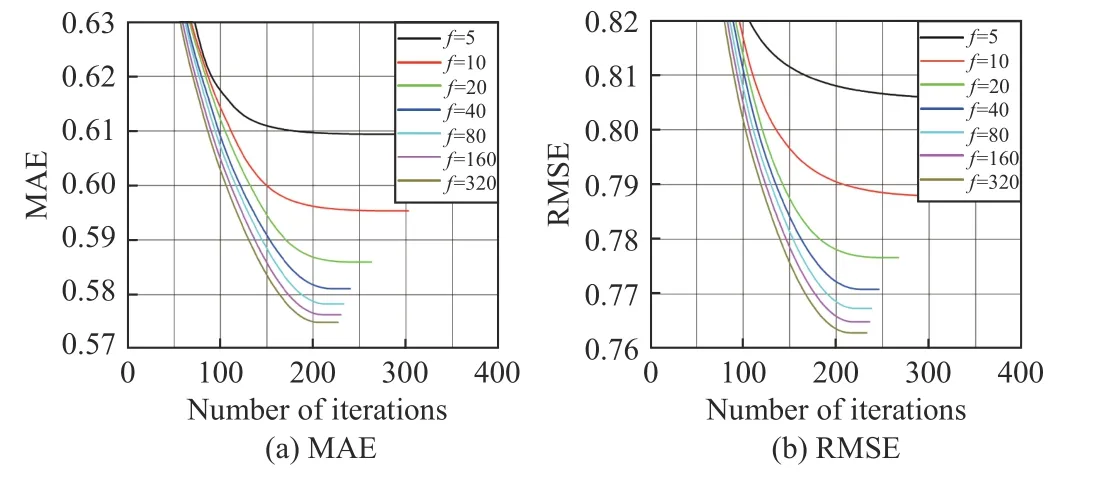
Fig.3. The training process of SL-LFb with different f on D8, where λ =0.01 and η = 0.001.
2) Impacts of λ and η
In this set of experiments, we increase λ from 0.01 to 0.1 and η from 0.0001 to 0.01 by performing a grid-based search [36]. Figs. 4 and 5 show the results on D8. The complete results on all the datasets are presented in the Supplementary File1. From them, we conclude that:

Fig.4. The experimental results of SL- LFb¯ with respect to λ and η on D8,where f = 20.

Fig.5. The experimental results of SL-LFb with respect to λ and η on D8,where f = 20.

TABLE II DESCRIPTIONS OF ALL THE COMPARISON MODELS
a) Both λ and η have a significant impact on prediction accuracy of both SL-L Fb¯and SL-LFb. As λ and η increase,MAE and RMSE decrease at first and then increase in general.For example, on D8, RMSE of SL-L Fb¯decreases from 0.8116 to 0.7729 at the beginning. Then, it increases up to 0.8451 as λ and η continue to increase.
b) λ and η have different situations in searching their optimal values on the tested datasets. On the different datasets, the optimal value of η is a small value like 0.001.However, the optimal value of λ is different for the different datasets. It distributes in the range from 0.02 to 0.09. Hence, λ should be carefully tuned on the target dataset.
C. Outlier Data Sensitivity Tests
In this section, we compare an SL-LF model with a basic LF (BLF) model when outlier data are added to the datasets.BLF is modeled based on the L2-norm-oriented Loss while SL-LF is done by the smooth L1-norm-oriented Loss. The specific method of adding outlier data is: 1) randomly selecting an unknown entity between two known entities as the outlier entity for the input HiDS matrix Z, 2) assigning a value (maximum or minimum known value) to the outlier entity, 3) the percentage that outlier entities account for known entities is increased from 0% to 100% with an interval of 10%, and 4) the outlier entities are only added into the training set. To illustrate this method, an example is given in Fig.6.
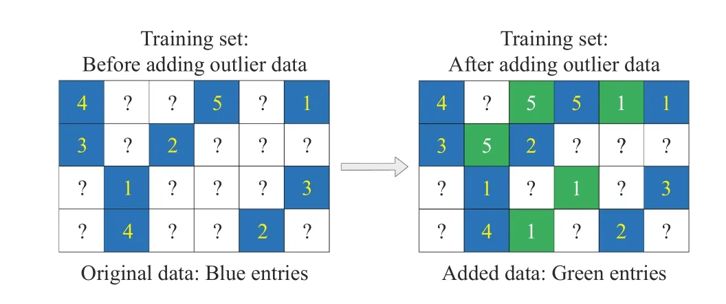
Fig.6. An example of adding outlier data.
Fig.7 records the experimental results on D8.Supplementary File1records the complete results on all the datasets. Since smooth L1-norm is less sensitive to outlier data than L2-norm, we find that both SL-L Fb¯and SL-LFbbecome much more robust than BLF as the percentage of outlier data increases. For example, on D8, RMSEs of SL-L Fb¯and BLF are 0.7767 and 0.7761, respectively when there are no outlier data, and then become 0.8536 and 1.1244, respectively when the percentage of outlier data is 100%. The improvement of RMSE of BLF is 0.3483, which is about 4.53 times as large as that of SL-L Fb¯at 0.0769. Therefore, we conclude that an SLLF model is robust to the outlier data.

Fig.7. The outlier data sensitivity tests results of BLF, SL- LFb¯,and SL-LFb on D8, where λ = 0.01, η = 0.001, and f = 20.
D. Comparison Between SL-LF and State-of-the-Art Models
We compare an SL-LF model with five related state-of-theart models, including three LF-based models (basic latent factor (BLF), non-negative latent factor (NLF), and fast nonnegative latent factor (FNLF)) and two deep neural network(DNN)-based models (AutoRec and deep collaborative conjunctive recommender (DCCR)). Table II gives a brief introduction to these models. To make a fair comparison, f is set as 20 for all the LF-based models and the proposed SL-LF model. Besides, we tune the other hyper-parameters for all the involved models to make them achieve their highest prediction accuracy.
1) Comparison of Prediction Accuracy
Table III presents the detailed comparison results. Statistical analysis is conducted on these comparison results. First, the win/loss counts of SL-L Fb¯/SL-LFbversus other models are summarized in the third/second-to-last row of Table III.Second, we perform Friedman test [40] on these comparison results. The result is recorded in the last row of Table III,where it accepts the hypothesis that these comparison models have significant differences with a significance level of 0.05.From these comparisons and statistical results, we find that a)both SL-L Fb¯and SL-LFbachieve lower RMSE/MAE than the other models on most testing cases, and b) SL-LFbachieves the lowest F-rank value among all the models. Hence, we conclude that SL-LFbhas the highest prediction accuracyamong all the models.

TABLE III THE COMPARISON RESULTS ON PREDICTION ACCURACY, INCLUDING WIN/LOSS COUNTS STATISTIC AND FRIEDMAN TEST, WHERE ●AND ✪RESPECTIVELY INDICATE THAT SL- LFb¯ , AND SL- LFb HAVE A HIGHER PREDICTION ACCURACY THAN COMPARISON MODELS
Next, we check whether SL-LFbachieves significantly higher prediction accuracy than each single model. To do so,we conduct the Wilcoxon signed-ranks test [41], [42] on the comparison results of Table III. Wilcoxon signed-ranks test is a nonparametric pairwise comparison procedure and has three indicators – R+, R−, and p-value. The larger R+ value indicates higher performance and the p-value indicates the significance level. Table IV records the test results, where we see that SL-LFbhas a significantly higher prediction accuracy than all the comparison models with a significance level of 0.05 except for SL-L Fb¯. However, SL-LFbachieves a much larger R+ value than SL-L Fb¯, which verifies that linear biases can boost an SL-LF model’s prediction accuracy.
2) Comparison of Computational Efficiency
To compare the computational efficiency of all the tested models, we measure their CPU running times on all the datasets. Fig.8 presents the results. From it, we observe that:
a) DNN-based models (AutoRec and DCCR) cost much more CPU running time than the other models due to their time-consuming DNN-based learning strategy [43].
b) SL-LF costs slightly more CPU running time than BLF.The reason is that SL-LF has the additional computational procedures of discrimination (11) while BLF does not.
c) SL-LF costs less or more CPU running time than NLF and FNLF on the different datasets.
Therefore, these results verify that SL-LF’s computational efficiency is higher than those of DNN-based models and comparable to those of other LF-based models.

TABLE IV STATISTICAL RESULTS ON TABLE III BY CONDUCTING THE WILCOXON SIGNED-RANKS TEST

Fig.8. The comparison CPU running time of involved models on D1–D8.
E. Summary of Experiments
Based on the above experimental results and analyses, we have the following conclusions:
1) An SL-LF model’s prediction accuracy is closely connected with λ and η. As a rule of thumb, we can set η=0.001 while λ should be fine-tuned according to a specific target dataset.
2) SL-LF has significantly higher prediction accuracy than state-of-the-art models for the missing data of an HiDS matrix.
3) SL-LF’s computational efficiency is much higher than those of DNN-based models and comparable to those of most efficient LF-based models.
4) Linear biases have positive effects on improving SL-LF’s prediction accuracy.
V. RELATED WORK
An LF model is one of the most popular and successful ways to efficiently predict the missing data of an HiDS matrix[13], [14]. Up to now, various approaches are proposed to implement an LF model, including a bias-based one [14], nonnegativity-constrained one [15], randomized one [17],probabilistic one [44], dual-regularization-based one [45],posterior-neighborhood-regularized one [16], graph regularized one [18], neighborhood-and-location integrated one [6],data characteristic-aware one [35], confidence-driven one[46], deep-latent-factor based one [47], and nonparametric one[48]. Although they are different from one another in terms of model design or learning algorithms, they all adopt an L2-norm-oriented Loss, making them sensitive to outlier data[20]. Since outlier data are frequently found in an HiDS matrix [24], [25], their robustness cannot be guaranteed.
To make an LF model less sensitive to outlier data, Zhu et al. [19] proposed to adopt an L1-norm-oriented Loss.However, such an LF model is multimodal because L1norm is less smooth than L2norm, as shown in Fig.1(a). Hence, an LF model with an L1norm-oriented Loss tends to be stacked by some “bad” solutions, resulting in its failure to achieve high prediction accuracy. Differently from these approaches, the proposed SL-LF model adopts smooth L1-norm-oriented Loss,making its solution space smoother and less multimodal than that of an LF model with L1norm-oriented Loss. Meanwhile,its robustness is also higher than that of an LF model with L2norm-oriented Loss.
Recently, DNN-based approaches to represent an HiDS matrix have attracted extensive attention [49]. According to a recent review regarding DNN-based studies [34], various models are proposed to address the task of missing data prediction for an HiDS matrix. Representative models include an autoencoder-based model [37], hybrid autoencoder-based model [39], multitask learning framework [50], neural factorization machine [51], attentional factorization machine[52], deep cooperative neural network [53], and convolutional matrix factorization model [54]. However, DNN-based models have the limit of high computational cost caused by their learning strategies. For example, they take complete data rather than known data of an HiDS matrix as input.Unfortunately, an HiDS matrix generated by RSs commonly has a very low rating density. In comparison, SL-LF trains only on the known data of an HiDS matrix, thereby achieving highly computational efficiency.
As analyzed in [13], [16], an LF model can not only predict the missing data of an HiDS matrix but also be used as a data representation approach. Hence, SL-LF has some potential applications in representation learning, such as community detection, autonomous vehicles [5], and medical image analysis [55]–[57]. Besides, some researchers incorporate non-negative constraints into an LF model to improve its performance [17]. Similarly, we plan to improve SL-LF by considering non-negative constraints [58] in the future.
VI. CONCLUSIONS
This study proposes, for the first time, a smooth L1-normoriented latent factor (SL-LF) model to robustly and accurately predict the missing data of a high-dimensional and sparse (HiDS) matrix. Its main idea is to employ smooth L1-norm rather than L2-norm to form its Loss (the error between observed data and predicted ones), making it achieve highly robust and accurate prediction of missing data in a matrix.Extensive experiments on eight HiDS matrices from industrial applications are conducted to evaluate the proposed model.The experimental results verify that 1) it is robust to the outlier data, 2) it significantly outperforms state-of-the-art models in terms of prediction accuracy for the missing data of an HiDS matrix, and 3) its computational efficiency is much higher than those of DNN-based models and comparable to those of most efficient LF models. Although it has shown promising prospects, how to make its hyper-parameter λ selfadaptive and improve its performance by considering nonnegative constraint remains open. We plan to fully investigate these issues in the future.
杂志排行
IEEE/CAA Journal of Automatica Sinica的其它文章
- Dynamic Evaluation Strategies for Multiple Aircrafts Formation Using Collision and Matching Probabilities
- Task Scheduling for Multi-Cloud Computing Subject to Security and Reliability Constraints
- Vibration Control of a High-Rise Building Structure: Theory and Experiment
- Residual-driven Fuzzy C-Means Clustering for Image Segmentation
- Decoupling Adaptive Sliding Mode Observer Design for Wind Turbines Subject to Simultaneous Faults in Sensors and Actuators
- Property Preservation of Petri Synthesis Net Based Representation for Embedded Systems
