WEIGHTED LASSO ESTIMATES FOR SPARSE LOGISTIC REGRESSION:NON-ASYMPTOTIC PROPERTIES WITH MEASUREMENT ERRORS∗
2021-04-08HuameiHUANG黄华妹
Huamei HUANG(黄华妹)
Department of Statistics and Finance,University of Science and Technology of China,Hefei 230026,China E-mail:huanghm@mail.ustc.edu.cn
Yujing GAO(高钰婧)
Guanghua School of Management,Peking University,Beijing 100871,China E-mail:jane.g1996@pku.edu.cn
Huiming ZHANG(张慧铭)
School of Mathematical Sciences,Peking University,Beijing 100871,China E-mail:zhanghuiming@pku.edu.cn
Bo LI(李波)†
School of Mathematics and Statistics,Central China Normal University,Wuhan 430079,China E-mail:haoyoulibo@163.com
Abstract For high-dimensional models with a focus on classification performance,the ℓ1-penalized logistic regression is becoming important and popular.However,the Lasso estimates could be problematic when penalties of different coefficients are all the same and not related to the data.We propose two types of weighted Lasso estimates,depending upon covariates determined by the McDiarmid inequality.Given sample size n and a dimension of covariates p,thefinite sample behavior of our proposed method with a diverging number of predictors is illustrated by non-asymptotic oracle inequalities such as the ℓ1-estimation error and the squared prediction error of the unknown parameters.We compare the performance of our method with that of former weighted estimates on simulated data,then apply it to do real data analysis.
Key words logistic regression;weighted Lasso;oracle inequalities;high-dimensional statistics;measurement error
1 Introduction
In recent years,with the advancement of modern science and technology,high-throughput and non-parametric complex data has been frequently collected in gene-biology,chemometrics,neuroscience and other scientific fields.With the massive data in regression problem,we encounter a situation in which both the number of covariates p and sample size n are increasing,and p is a function of n,i.e.,p=:p(n).One further assumption in the literature is that p is allowed to grow with n but p ≤n,this has been extensively studied in works(see [9,19,27,28]and references therein).When we consider the variable selection in terms of a linear or generalized linear model,massive data sets bring researchers unprecedented computational challenges,such as the“large p,small n”paradigm;see [16].Therefore,another potential characterization appearing in large-scale data is that we only have a few significant predictors among p covariates and p ≫n.The main challenge is that directly utilizing low-dimensional (classical and traditional) statistical inference and computing methods for this increasing dimension data is prohibitive.Fortunately,the regularized(or penalized) method can perform parameter estimation and variable selection to enhance the prediction accuracy and interpretability of the regression model it generates.One famous proposed method is the Lasso (least absolute shrinkage and selection operator) method,which was introduced in [21]as modification of the least square method in the case of linear models.


where Y∈{0,1}is the response variable of the individual i,and βis a p×1 vector of unknown regression coefficients belonging to a compact subset of R.The unknown parameter βis often estimated by the maximum likelihood estimator (MLE) through maximizing the log-likelihood function with respect to β,namely,

For more discussions of binary response regression,we refer readers to [20]for a comprehensive introduction,and to [8]for a refreshing view of modern statistical inference in today’s computer age.
In the high-dimensional case,we often encounter a situation where the number of predictors p is larger than the sample size n.When p ≫n,the least square method leads to overparameterization;Lasso and many other regularization estimates are required to obtain a stable and satisfactory fitting.Although the Lasso method performs well,some generalized penalities have been proposed,since researchers want to compensate for certain of Lasso’s shortcomings,and to make the penalized method more useful for a particular data set;see [12].Since Lasso gives the same penalty for each β,an important extension is to use different levels of penalties to shrink each covariate’s coefficients.The weighted Lasso estimation method is an improvement of Lasso,where penalized coefficients are estimated based on different data-related weights,but one challenge is that this weighted method depends on both covariates and responses,so it is difficult for us to find the optimal weights.

• This paper proposes the concentration-based weighted Lasso for inference high dimensional sparse logistic regressions;the proposed weights are better than [15]in terms of applications.
• This paper derives the non-asymptotic oracle inequalities with a measurement error for weighted Lasso estimates in sparse logistic regressions,and the obtained oracle inequalities are shaper than [5]in the case of Lasso estimates of logistic regressions.
• The Corollary 2.1 is the theoretical guarantee when we do a simulation;the smallest signal should be larger than a threshold value.
This paper is organized as following:in Section 2,the problem of estimating coefficients in a logistic regression model by weighted Lasso is discussed,and we give non-asymptotic oracle inequalities for it under the Stabil Condition.In Section 3,we introduce novel data dependent weights for Lasso penalized logistic regression and compare this method with other proposed weights.Our weights are based on the KKT conditions such that the KKT conditions hold with high probability.In Section 4,we use a simulation to show how our proposed methods can rival the existing weighted estimators,and apply our methods for a real genetic data analysis.
2 Weighted Lasso Estimates and Oracle Inequalities
2.1 ℓ1-penalized sparse logistic regression
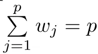
We consider the following estimator of ℓ-penalized logistic regression




The gradient of ℓ(β) is


Theoretically,the data-dependent turning parameter λwis required to ensure that the KKT conditions evaluated at the true parameter hold with high probability.In section 3,we will apply McDiarmid’s inequality of the weighted sum of random variables to obtain λw.In addition,McDiarmid’s inequality is an important ingredient that can help us establish the oracle inequality for the weighted Lasso estimate in the next section.
2.2 Oracle inequalities
Deriving oracle inequalities is a powerful mathematical tool which provides deep insight into the non-asymptotic fluctuation of an estimator in comparation with the ideal unknown estimate,which is called oracle.A comprehensive theory of high-dimensional regression has been developed for Lasso and its generalization.Chapter 6 of[3]and Chapter 11 of[12]outline the theory of Lasso,including works on oracle inequalities.In this section,non-asymptotic oracle inequalities for the weighted Lasso estimate of logistic regression are sought,under the assumptions of the Stabil Condition.
Before we get to our arguments,we first introduce the definition of Stabil Condition (a type of restricted eigenvalue originally proposed in[2]),which provides a tuning parameter and sparsity-dependent bounds for the ℓ-estimation error and the square prediction error.Most importantly,we consider the following two assumptions:


Although there are applications where unbounded covariates will be of interest,for convenience,we do not discuss the case with unbounded covariates.We also limit our analysis to bounded predictors,since the real data we collected was often bounded.If data is not bounded,we can take a log-transformation of the original data,thus making the transformed data almost bounded,We can also establish transformation f(X)=exp(X)/{1+exp(X)};thus the transformed predictors are undoubtedly bounded variables.
Let βbe the true coefficient,which is defined by minimization of the unknown risk function

where l(Y,X;β)=−Y Xβ+log{1+exp(Xβ)} is the logistic loss function.
It can be shown that(2.3)coincides(1.1).The first order condition for convex optimization(2.3) is


To establish the desired oracle inequalities,on WC(k,ε) we assume that the p×p matrix Σ=E(XX) satisfies at least one of the following conditions:the Stabil Condition (see [5]) or the Weighted Stabil Condition (our proposed condition).
Definition 2.1
(Stabil Condition) For a given constant c>0 and the measurement error ε>0,let Σ=E(XX) be a covariance matrix,which satisfies the Stabil condition S(c,ε,k)if there exists 0
for any b ∈WC(k,ε).
Definition 2.2
(weighted Stabil Condition) For a given constant c>0 and the measurement error ε >0,let Σ=E(XX) be a covariance matrix,which satisfies the Weighted Stabil condition WS(c,ε,k) if there exists 0
for any b ∈WC(k,ε).
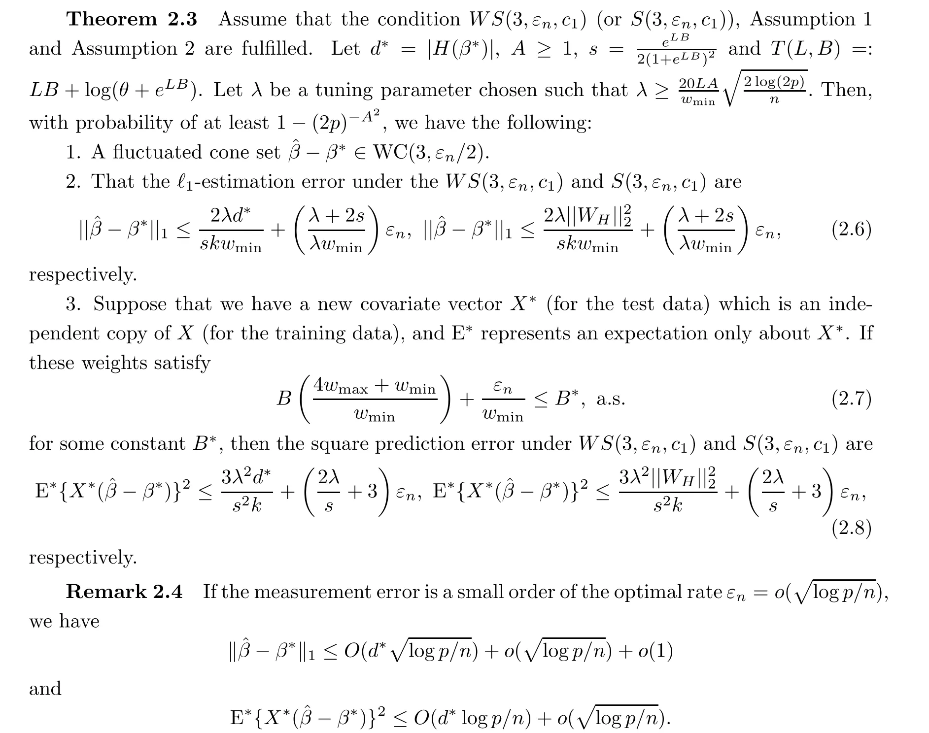
The constants c,cin the above two conditions are essentially the lower bound on the restricted eigenvalues of the covariance matrix.For convenience,we use the same ε in the above two conditions and in the weighted cone set.Under the above mentioned assumptions,we have the following oracle inequalities:

Remark 2.5
If (2.1) is replaced by the robust penalized logistic regression(see [17,24])as
where Ris some weight such that nR≤C in the weighted log-likelihood(here C is a constant),then we still have oracle results similar to Theorem 2.3.

The proof of Theorem 2.3 and the ensuing corollary are both given in Section 5.

Corollary 2.7
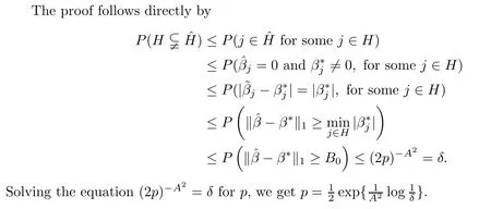
Let δ ∈(0,1) be a fixed number.Suppose that the assumption of Theorem 2.3 is satisfied,and the weakest signal and strongest signal meet the condition
This corollary is the theoretical guarantee when we do a simulation that the smallest signal of βshould be large such that we have a threshold value which is also called the Beta-min Condition (see [3]).
3 Data-dependent Weights

Lemma 3.1
Suppose that X,···,Xare independent random variables all taking values in the set A,and assume that f :A→R is a function satisfying the bounded difference condition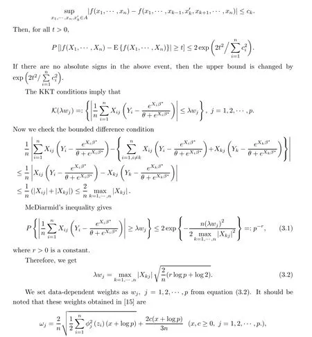

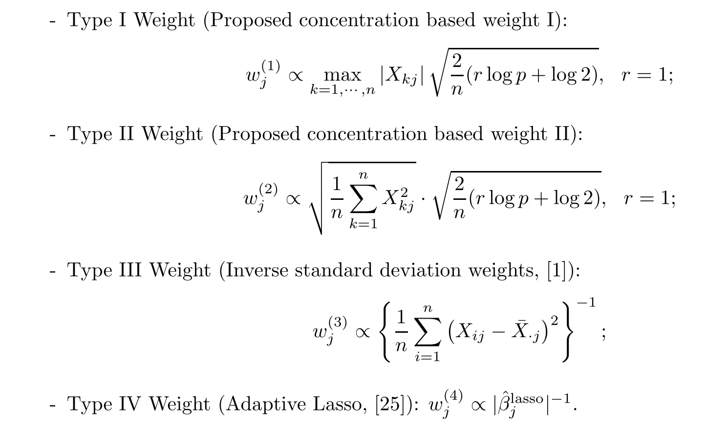
One may also find a more particular way to define weights in references.In high-dimensional settings,unlike those for the previously proposed weighted Lasso estimates,our weights are based on conditions which hold with high probability.Various weights that we compare in the next section are:
4 Simulation and Real Data Results
4.1 Simulation Results
In this section,we compare the performance of the ordinary Lasso estimate and the weighted Lasso estimate of logistic regression on simulated data sets.We use the R package glmnet with function glmreg() to fit the ordinary Lasso estimate of logistic regression.For the weighted Lasso estimate,we first apply function cv.glmnet() for 10-fold cross-validation to obtain the optimal tuning parameter λ.The actual weights we use are the standardized weights given by
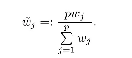
Then we transfer our weighted problem into an unweighted problem and apply the function lbfgs() in R package lbfgs to find the solution for the unweighted Lasso optimal problem.The original weighted optimal problem is


A Data generation
For each simulation,we set n=100 and n=200.We set the dimensions as p=50,100,150 and 200,and adopt the simulation setting as the following two patterns:
1.The predictor variables X are randomly drawn from the multivariate normal distribution N(0,Σ),where Σ has elements ρ(k,l=1,2,···,p).The correlation among predictor variables is controlled by ρ with ρ=0.3,0.5 and 0.8.We assign the true coefficient parameter of logistic regression as

2.Similar to case 1,we generate predictor variables X from multivariate normal distribution N(0,Σ),where Σ has elements ρ(k,l=1,2,···,p),and ρ=0.3,0.5 and 0.8,and we set the true coefficient parameter as

B Simulation results
These simulation results are listed in Tables 1 to 3.
From these simulation results,our proposed estimate with Type II weight is better than other methods in most cases,both in terms as ℓ-error and prediction error.The adaptive Lasso estimate performs worst among these five ℓ-penalized estimates.
4.2 Real Data Results
In this section,we apply our proposed estimates to analyze biological data.We consider the following two complete data sets:
(a)The first data set is the gene expression data from a leukemia microarray study(see[10]).The data comprises n=72 patients,in which 25 patients have acute myeloid leukemia (AML)and 47 patients have acute lymphoblastic leukemia(ALL).Therefore,the binary response in this data set is categorized as AML (label 0) and ALL (label 1).The predictors are the expression levels of p=7129 genes.The data can be found in R package golubEsets.
(b) The second data set is the above gene expression data after preprocessing and filtering(see [7]).This process reduces the number of genes to p=3571.The data set can be found in R package cancerclass.
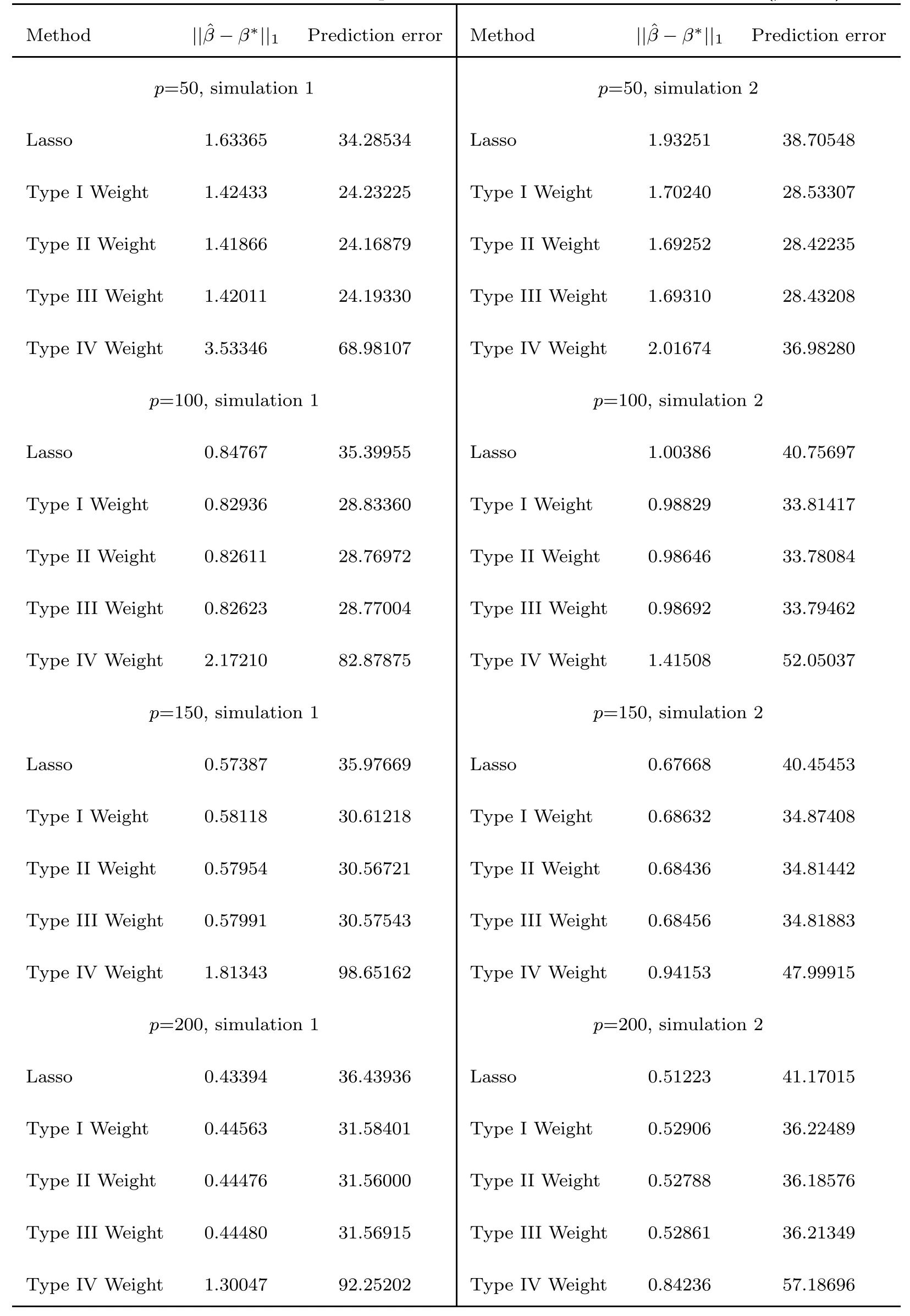
Table 1 Means of ℓ1-error and prediction error for simulation 1 and 2 (ρ=0.3)
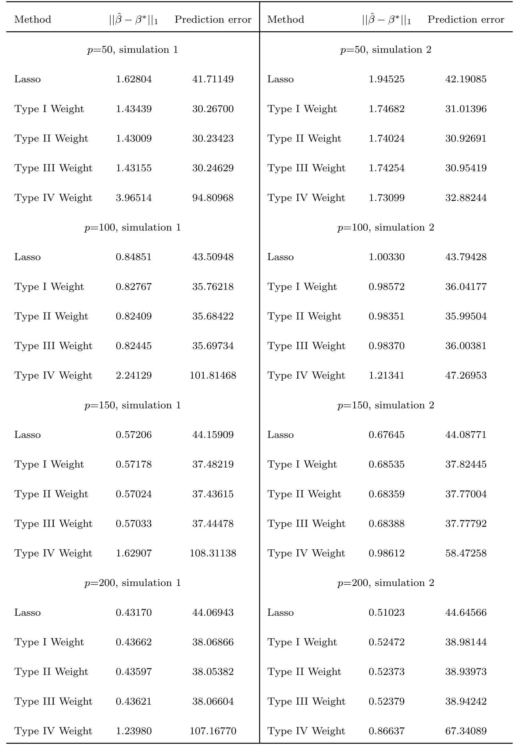
Table 2 Means of ℓ1-error and prediction error for simulation 1 and 2 (ρ=0.5)
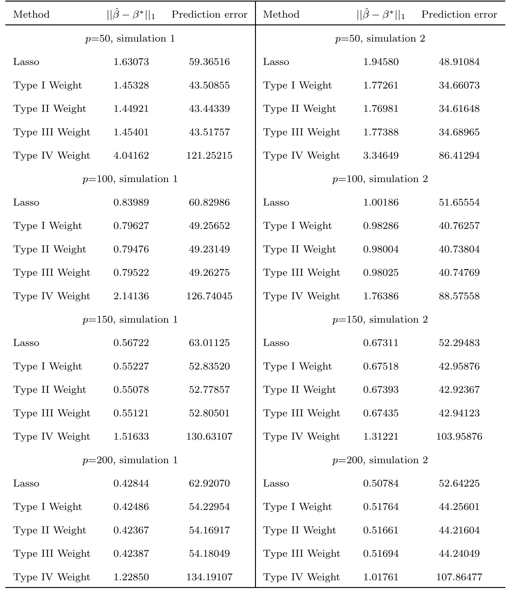
Table 3 Means of ℓ1-error and prediction error for simulation 1 and 2 (ρ=0.8)
Our target is to select useful genes for specifying AML and ALL.Note that there is no available information about model parameters,so we cannot directly compare the selection accuracy and prediction accuracy.Therefore,we list model size and the prediction error of the estimated model under the Leave-One-Out Cross-Validation(LOOCV) framework.Model size can show the coverage of the current estimated model,prediction error can show the prediction accuracy.We apply the ordinary Lasso method and four different weighted Lasso methods as described in the previous section to analyze these data sets.Since lots of coefficients estimated by weighted Lasso methods are small but not zero,we choose 10and 10as the limits for these two data sets separately,and set the coefficients that are less than these limits to zero.These results are summarized in Table 4.
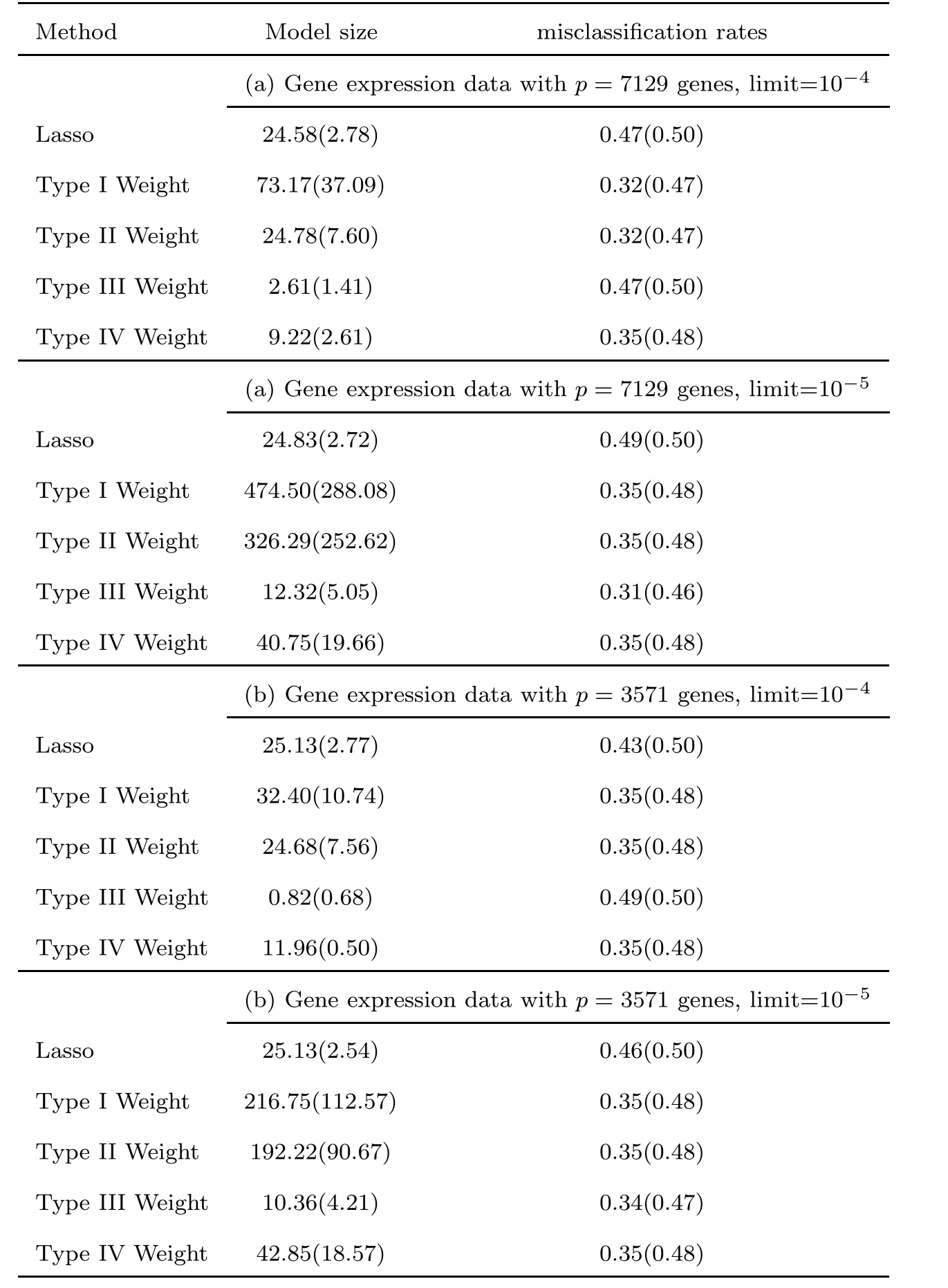
Table 4 Mean and standard deviation of model size and misclassification rate under Leave-One-Out Cross-Validation framework
In the first data set with limit 10,the weighted Lasso estimate with Type II Weight has the best prediction performance;in the first data set with limit 10,the weighted Lasso estimate with weight Type III Weight has the best prediction performance.In the second data set with limit 10,the weighted Lasso estimates with Type I Weight,Type II Weight and Type IV Weight have a similar prediction performance,and the weighted Lasso estimates with Type II Weight and Type IV Weight use less predictor variables than other methods;in the second data set with limit 10,the weighted Lasso estimate with Type III Weight has the best prediction performance and also uses the fewest variables.Therefore,we can see that the weighted Lasso method with Type II Weight,Type III Weight and Type IV Weight can estimate more accurately and with less predictors than other methods.
After comparing these five methods,we build a model for the complete observations,and report the selected genes in ordinary Lasso regression and some weighted Lasso methods which have small LOOCV errors.These results are listed in Tables 5 and 6.We observe that the weighted Lasso estimate with Type II Weight selects more variables than the weighted Lasso estimates with Type III and Type IV Weights,and has less refitting prediction errors.Summarizing the above results,our proposed weighted Lasso method can pick much more meaningful variables for explanation and prediction.

Table 5(a) Genes associated with ALL and AML selected by four methods (p=7129)
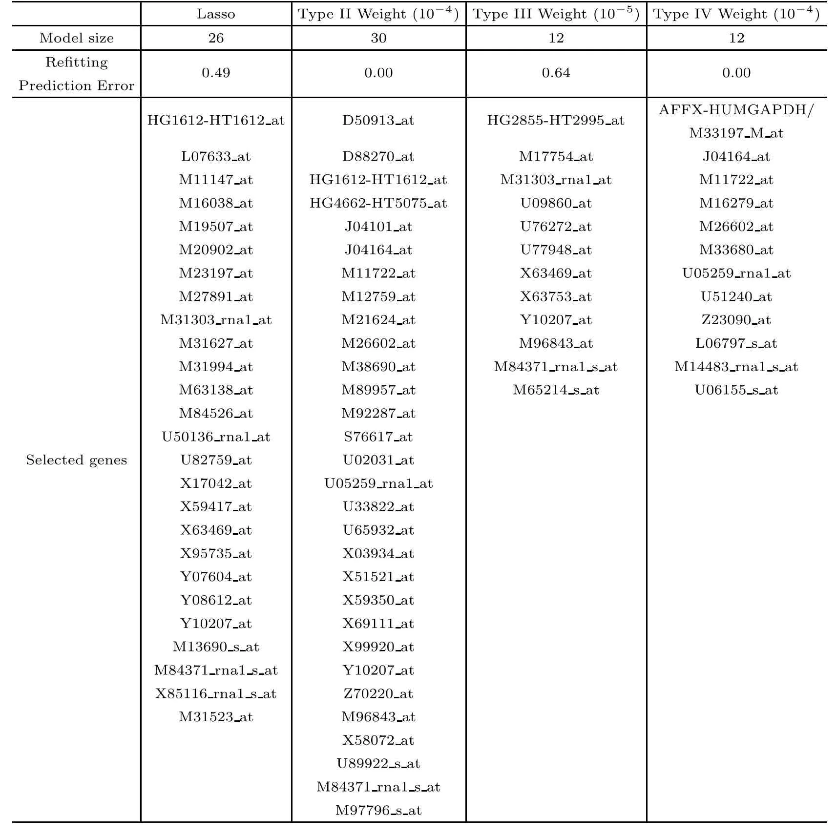
Table 6(b) Genes associated with ALL and AML selected by four methods (p=3571)
5 Proofs
5.1 The Proof of Theorem 2.3
The non-asymptotic analysis of Lasso and its generalization often leans on several steps.
The first step is to propose a restricted eigenvalue condition or other analogous condition about the design matrix,which guarantees local orthogonality via a restricted set of coefficient vectors.
The second step is to get the size of tuning parameter based on KKT optimality conditions(or other KKT-like condition such as Dantzig selector).

The language our proof is heavily influenced by theory of empirical process.For simplicity,we denote the theoretical risk by Pl(β)=:E{l(y,β,X)} and the empirical risk by
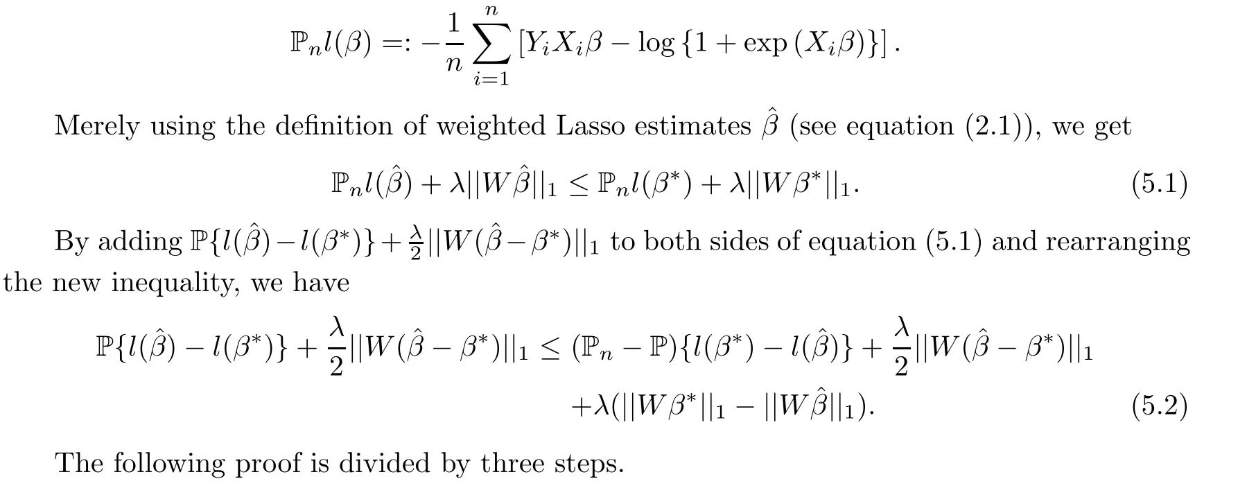
5.2 Step 1:Choosing the order of tuning parameter
Define the following stochastic Lipschitz constant in terms of the suprema of a centralized empirical process:


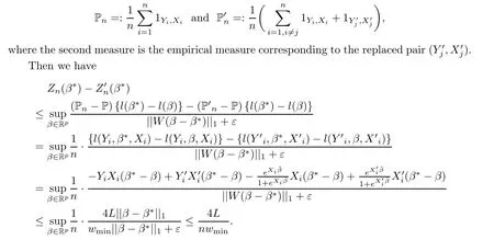
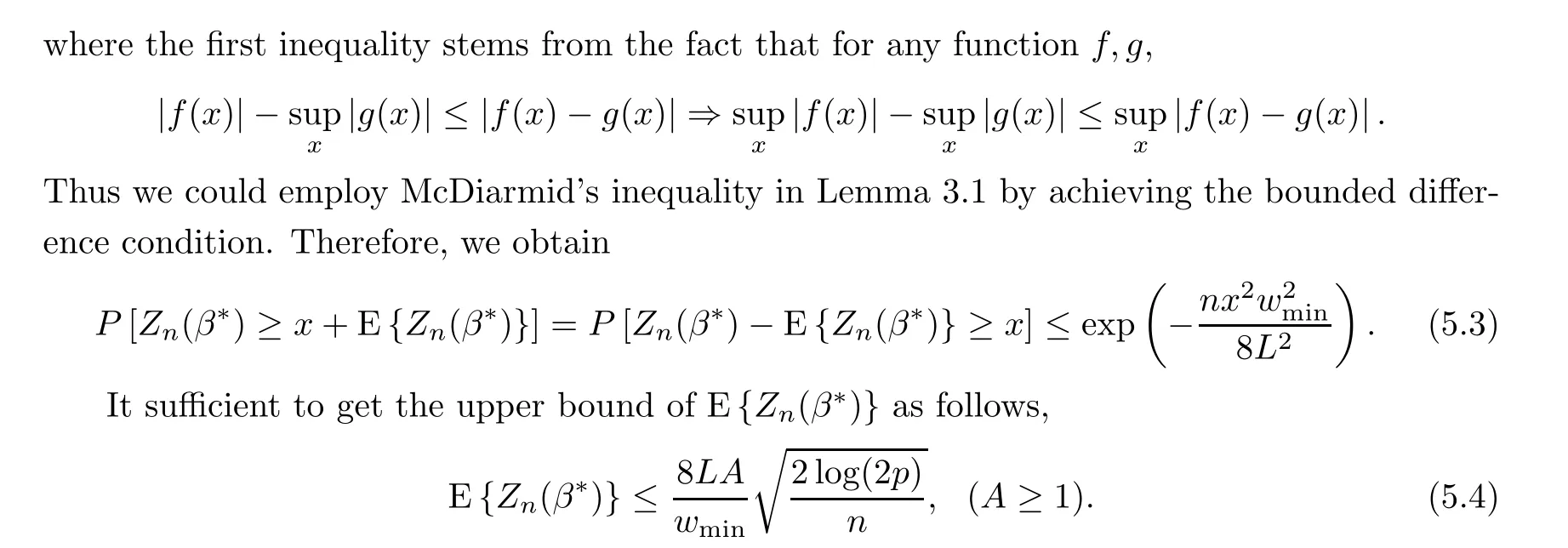
To obtain (5.4),we need the next two lemmas.The proof of the ensuring symmetrization and contraction theorems can be found in Section 14.7 of [3].
Let X,···,Xbe independent random variables taking values in some space X,and let F be a class of real-valued functions on X.
Lemma 5.1
(symmetrization theorem) Let ε,···,εbe a Rademacher sequence with uniform distribution on {−1,1},independent of X,···,Xand f ∈F.Then we have
where E[·]refers to the expectation w.r.t.X,···,Xand E{·} w.r.t.ǫ,···,ǫ.
Lemma 5.2
(contraction theorem) Let x,···,xbe the non-random elements of X and let ε,···,εbe a Rademacher sequence.Consider c-Lipschitz functions g,i.e.,


Thus the function ghere is 2-Lipschitz (in the sense of Lemma 5.2).
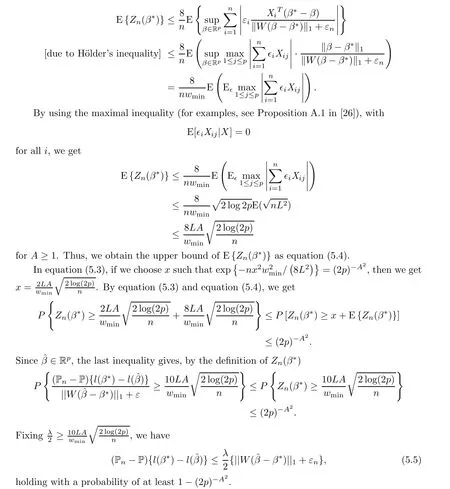
Apply the symmetrization theorem and the contraction theorem implies
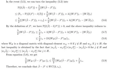
5.3 Step 2:Check −β∗∈WC(3,εn)
5.4 Step 3:Derive error bounds from Stabil Condition
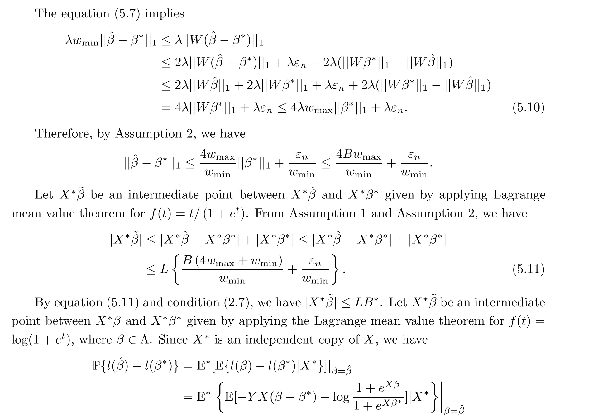
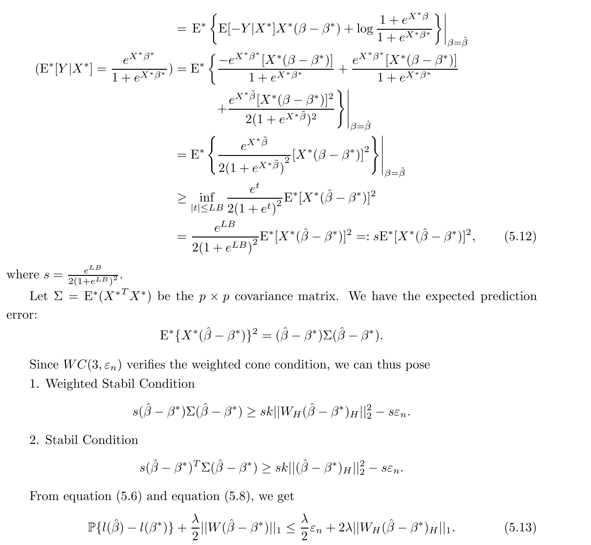
5.4.1 Case of the Weighted Stabil Condition
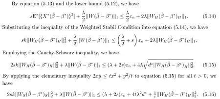
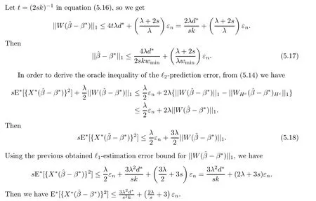
5.4.2 Case of the Stabil Condition
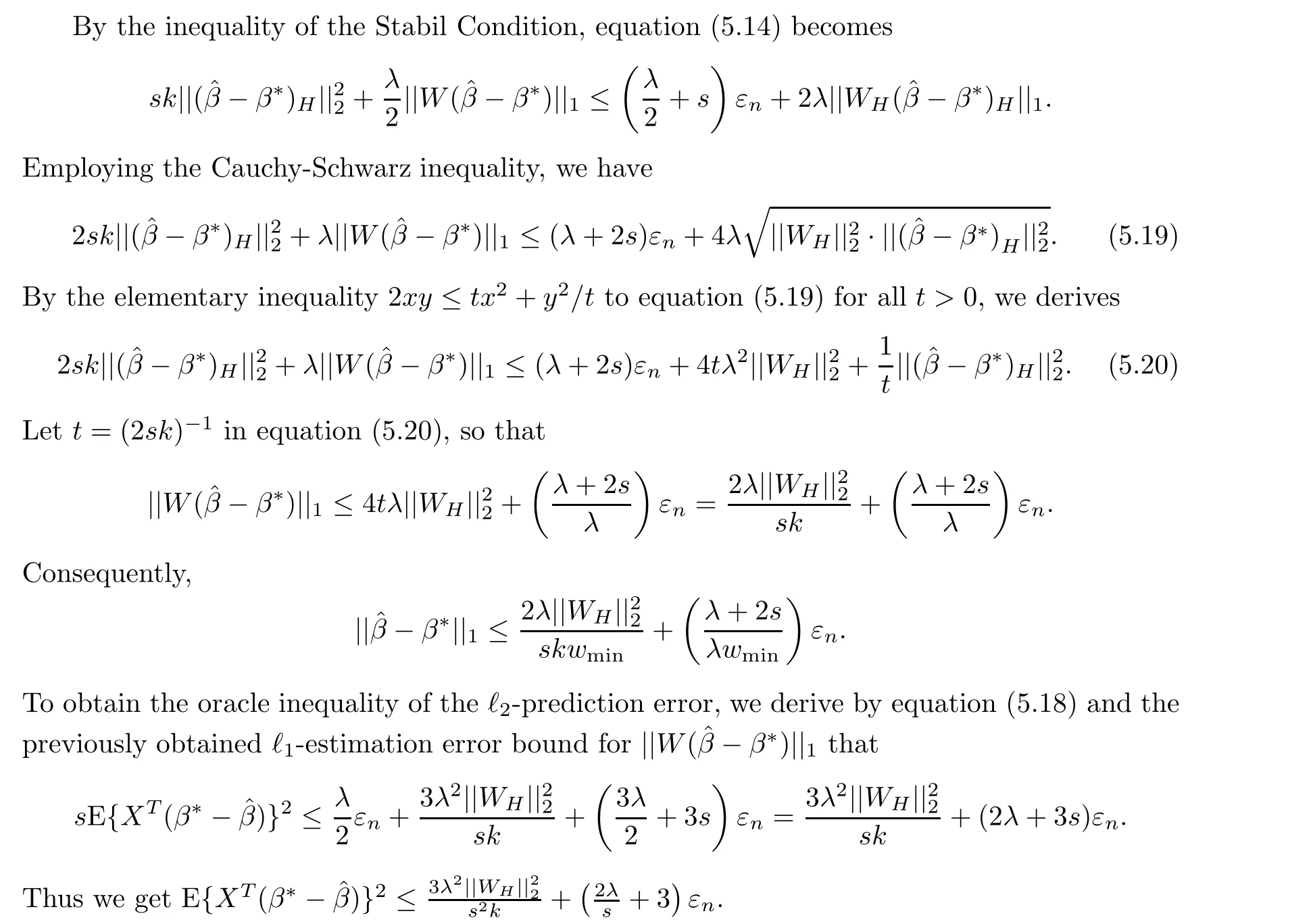
5.5 Proof of Corollary 2.7
6 Summary

杂志排行
Acta Mathematica Scientia(English Series)的其它文章
- CONTINUOUS DEPENDENCE ON DATA UNDER THE LIPSCHITZ METRIC FOR THE ROTATION-CAMASSA-HOLM EQUATION∗
- WEAK SOLUTION TO THE INCOMPRESSIBLE VISCOUS FLUID AND A THERMOELASTIC PLATE INTERACTION PROBLEM IN 3D∗
- ISOMORPHISMS OF VARIABLE HARDY SPACES ASSOCIATED WITH SCHRÖDINGER OPERATORS∗
- HITTING PROBABILITIES OF WEIGHTED POISSON PROCESSES WITH DIFFERENT INTENSITIES AND THEIR SUBORDINATIONS∗
- INHERITANCE OF DIVISIBILITY FORMS A LARGE SUBALGEBRA∗
- SOME SPECIAL SELF-SIMILAR SOLUTIONS FOR A MODEL OF INVISCID LIQUID-GAS TWO-PHASE FLOW∗
