Intrinsic component filtering for fault diagnosis of rotating machinery

Zongzhen ZHANG, Shunming LI, Jiantao LU, Yu XIN, Huijie MA

College of Energy and Power Engineering, Nanjing University of Aeronautics and Astronautics, Nanjing 210016, China

KEYWORDS Compound fault separation;Intelligent fault diagnosis;Intrinsic component filtering;Unsupervised learning;Weak signature detection

Abstract Fault diagnosis of rotating machinery has always drawn wide attention. In this paper,Intrinsic Component Filtering (ICF), which achieves population sparsity and lifetime consistency using two constraints: l1/2 norm of column features and l3/2 -norm of row features, is proposed for the machinery fault diagnosis.ICF can be used as a feature learning algorithm,and the learned features can be fed into the classification to achieve the automatic fault classification.ICF can also be used as a filter training method to extract and separate weak fault components from the noise signals without any prior experience. Simulated and experimental signals of bearing fault are used to validate the performance of ICF. The results confirm that ICF performs superior in three fault diagnosis fields including intelligent fault diagnosis, weak signature detection and compound fault separation.

1. Introduction

Big data promise to bring perspectives and challenges in the fault diagnosis and condition monitoring of rotating machinery.1Unsupervised learning-based diagnosis methods, which can reduce the dependence on human labor and make condition monitoring and fault diagnosis easier in big data environments, have been widely applied in rotating machinery fault diagnosis.2

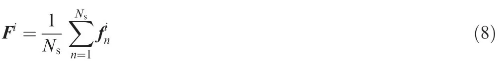
Unsupervised learning methods have recently become an important tool in intelligent fault diagnosis including Stacked Auto-Encoders (SAE),3,4Sparse Filtering (SF),5and Restricted Boltzmann Machines (RBMs).6,7Unsupervised learning methods are used to adaptively learn discriminative features from row signals.These features are fed to a classifier to diagnose the fault conditions.Lei et al.proposed a diagnosis method for fault diagnosis of machines constructed by SF and softmax regression.2In Ref.8,General Normalized Sparse Filtering (GNSF) is developed and the properties of normalization parameters are studied and discussed. In Ref.9, stacked denoising autoencoders with three hidden layers are used for rotating machinery fault diagnosis. Wang et al. proposed the batch-normalized deep neural networks to improve the training efficiency and diagnostic accuracy.10It should be noted that SF has the merits of simplicity and high efficiency. Unsupervised learning methods can also be used to solve other problems. Independent Component Analysis (ICA) and its variants have been widely applied to the fault diagnosis such as multi-channel fault signal separation and compound fault separation.11,12Jia et al. proposed Convolutional Sparse Filtering (CSF) and developed its variants SF with the generalizedlp/lq-norm for impulsive feature enhancement.13,14

It can be found that unsupervised learning methods can be used to solve various fault diagnosis problems and have achieved good results.However,these methods and its application may suffer three weaknesses as follows. First, unsupervised learning is mainly to extract discriminative feature. In the absence of reconstructed term,such constraints often cause poor robustness in feature learning process for small sample set. Second, due to the fact that fault information is usually corrupted by the ambient noise, these methods face seriously performance degradation in practical application. Third, in the application of weak signature detection, signal separating method is necessary if there are multiple faults in one signal,which is time-consuming and largely dependent on much prior knowledge.

In this paper, to overcome the above shortcomings, Intrinsic Component Filtering (ICF) is proposed for rotating machinery fault diagnosis. To our best knowledge, this is the first attempt for solving three problems simultaneously including intelligent fault diagnosis, weak signature detection and compound fault separation. The main contributions of this paper can be summarized as follows. First, ICF can ensure the lifetime consistency between the same conditions and realize the lifetime sparsity between different conditions. Therefore, ICF can also be used to automatically learn the discriminative information from the raw data. Second, ICF shows superior noise adaptability and robustness in the application of weak signature detection, which could simultaneously process big data with multiple samples in noisy environment. Third, ICF can be regarded as a multi-channel blind deconvolution to enhance and separate weak fault information from the compound fault signals without any priori estimation.

The rest of this paper is organized as follows.Section 2 discusses the related works including weak signature detection,compound fault separation and unsupervised learning-based diagnosis method. Section 3 introduces the theoretical relationship between sparsity measure and normalization and details the proposed intrinsic component filtering. Sections 4-6 conduct and discuss three experiments using ICF.Finally,conclusions are drawn in Section 7.

2. Related work

The related works are described in this section containing the intelligent fault diagnosis, weak signature detection and compound fault diagnosis method.

2.1. Intelligent fault diagnosis

Given that the purpose of fault diagnosis is to identify the fault condition, a good representation of true data is not a strict requirement for a classification-oriented algorithm.Moreover,the algorithms without reconstructing term are more efficient because fewer parameters need to be adjusted. The characterization of unsupervised learning has been expressed as a way of modeling desired feature distribution,rather than the true representation of data.

Sparse filtering, in whichl2-normalization is used to obtain the population sparsity and lifetime sparsity,is an efficient and simple feature learning method that requires minimal tuning parameters 5. There are many studies and discussions on the application of SF in fault diagnosis. However, due to the fact that the characteristics of the faults with the same condition are often similar, the feature learning performance of SF will be greatly reduced when only one fault exists in the training samples. In practice, the consistency of feature distribution of samples with the same fault condition and the discrimination between different fault conditions are equally important to the accuracy and robustness of diagnostic result.

2.2. Weak signature detection

Weak signature detection of vibration signal in noisy environment is an important topic in the machine fault diagnosis.15,16Many methods have been proposed to enhance the impulsive signature of raw signal, such as Empirical Mode Decomposition (EMD),17,18Spectral Kurtosis (SK),19-21wavelet,22-23Minimum Entropy Deconvolution(MED),24-26Convolutional Sparse Filtering (CSF),8etc. EMD and its variants can effectively decompose the vibration signal into multiple different components in time domain. However, the performance of EMD will be discounted in the strong noisy environment.SK and wavelet decompose the vibration signal using the filter bank that needs to be defined in advance. MED and CSF approach this problem using sparse optimization, which regularize the sparsity of the input signal using maximization of the Kurtosis andl1/2-norms. The corresponding variants such as SF based on the generalizedlp/lq-norm and generalized MED developed the object function to the general form. Similar to unsupervised learning method, the emphasis of these methods is not to pursue the best inverse filters, but to learn the sparse features of input signals.

It is noticed that sparse optimization-based method has become a hotspot in the impulsive signature enhancement.Assume that an algorithm can extract sparse features, which are inherent components of the samples, and the trained weight matrix can be regarded as an inverse filter.

2.3. Compound fault separation

When the mechanical system fails, we do not stop the machines immediately, and the continuous operation of the equipment in a harsh environment may lead to a compound fault.27Compound fault diagnosis has become a hotspot and the key is the component separation of the compound fault signal.

Various methods are proposed for compound fault diagnosis, and some weak signature detection methods mentioned above could be used to separate compound fault diagnosis.28Morphological Component Analysis (MCA) approaches this problem from another way.29Generally, we need to choose a dictionary to accurately describe the characteristics of the fault. In Ref.30, Symmlet wavelets, Daubechies wavelets and Coiflet wavelets are used to extract the impulse component,and Local Discrete Cosine and Sine dictionaries (LDCS) are used to learn the meshing component. However, the suitable selection of dictionary is important for the separation performance of compound faults. In addition, there may be many kinds of impulse fault components produced by different compound faults. In this case, the dictionary that we choose will extract different shock signals as one fault. In Ref.31, Maximum Correlated Kurtosis Deconvolution (MCKD) is used to diagnose the compound bearing fault. However, the main problem in the practical application is that it requires a priori basis to set the parameters.32CSF can obtain multiple filters and separate compound faults;however the study on this area has not been carried out yet and the robustness of CSF is degraded in strong noisy environment.

3. Intrinsic component filtering

This section presents the proposed ICF. Firstly, the relationship between normalization and sparse constraints is discussed. Then, the construction process of the proposed ICF is detailed.

3.1. Normalization and sparse constraints

Sparsity is a core concept in machine learning, which means that a small number of significant features are activated to represent multi-dimensional samples. Sparse filtering achieves the discrimination and sparsity of the features by normalizing the rows and columns of the feature matrix usingl2-norms.

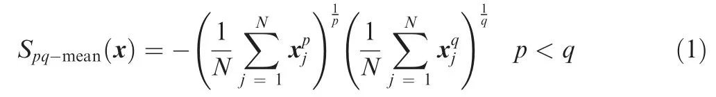
In Ref.33, Niall Hurley and Richard give the results that thepq-mean can satisfy all presented criteria whenp≤1 andq>1. Thepq-mean means the ratio of the generalizedlp-norm and thelq-norm, which refers to a group of meaningful sparse expressions. Thepq-mean can be expressed by

Jia et al. developed the sparse filtering to the generalizedlp/lq-norm and employed it to enhance impulsive signature.13The algorithm views the activation function as a convolution process.Recent Ref.3proposed the generalized normalization of sparse filtering for intelligent fault diagnosis, as shown in Eq. (3). The sparse optimization can be obtained using the minimization ofJgnsf（f） whenpq.

Normalization means constraints and competition between features. Take a special form ofpq-mean,l1/2-norm, as an example. The normalized features are constrained on thel2sphere. During the optimization process, competition between features is introduced. The normalized features are forced to move to the opposite coordinate axis.The ratio of the original features will be far from 1.

3.2. Proposed method

As mentioned above, a good unsupervised learning method can obtain a desired feature distribution. The ICF is proposed for rotating machinery fault diagnosis. ICF focuses on the consistency between the samples with the same fault condition. Thel1/2-norm of the column of feature matrix is used to realize the sparsity of features per sample and thel3/2norm of rows is used to achieve the consistency of features between samples.

where xi∈RN×1is the raw fault signals,Mmeans the number of samples, andmeans thejth feature of theith sample.(1) Population sparsity term. In the proposed method, thel1/2-norm is employed to measure the sparsity of features per sample.l2-norms of each column of the feature matrix are used to normalize corresponding column features.l1-norm of each normalized feature is considered as the population sparsity term.

(2) Lifetime consistency term. Thel3/2-norm of rows is used to achieve the consistency of features between samples.l2-norms of each raw of the feature matrix are used to normalize the corresponding row features. Cubic ofl3-norm of each normalized feature is used as the lifetime consistency term.

(3)Objective function.In order to eliminate the influence of redundancy in optimization process, the weight vectors are constrained.By integrating Eq.(4)and Eq.(5),the final objective function of ICF is written as

where λ>0 control the tradeoff between the two terms.

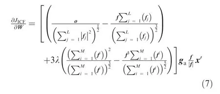
(4) Optimization process.JICFis nonconvex and nonsmooth, and f| | is replaced by the soft-absolute functionwhere ε is a small positive number. In this paper,the value of ε quals 1×10-8. The gradient function of the objective function can be given by where o ∈RL×Mis a matrix of all ones and gais the gradient of the activation function.

The procedure for the proposed ICF can be presented as Algorithm 1.

Algorithm 1.(L-BFGS procedure of the proposed ICF).

Feature matrix for training is constructed by the input samples.Repeating the following steps until the stopping criterion is met.Step 1. Calculate the gradient of the objective function through Eq. (7).Step 2. Update W using Limited-memory Broyden-Fletcher-Goldfarb-Shanno (L-BFGS): W（k） = W（k-1）-H-1 w gw, where H-1 w is the Hessian matrix estimated by L-BFGS algorithm.Step 3. Update f through feed forward f = Wx.

(5) Deep intrinsic component filtering. The proposed ICF can be developed for training deep networks using greedy layer-wised training. In this way, we can use the non-linear activation functionsto compute the features.The Deep Intrinsic Component Filtering (DICF) can be presented as in Algorithm 2.

Algorithm 2.(L-BFGS procedure for the proposed DICF).

Feature matrix for training is constructed by the input samples.Repeating the following steps until the stopping criterion is met.Step 1.Calculate the gradient of the objective function following Eq.(7)and obtain weighting matrix W1 of the Layer 1 following Algorithm 1.Step 2.Obtain the feature matrix for training the Layer 2 via feed forward f1 = W1x.Step 3. Obtain the weighting matrix W2 following Step 1.Step 4. Obtain the feature matrix of the Layer 2 f2 = W2f1 through Step 2.Step 5. Repeat the Steps 2-4 to train all of the layers.

(6) Characteristics ofl1/2-norm andl3/2-norm. To further explain the characteristics of intrinsic component filtering.Thel3/2-norm andl1/2-norm of a two-dimensional vector are shown in Fig. 1. The minimum value ofl3/2-norm is on the coordinate axis, which means that the value of a features is 0. However, the minimum value ofl3/2-norm is on the diagonal line, which means that the values of the two features are equal. As shown in Fig. 2(a), the column features tend to be sparse (f1=0，f2=1 orf2=0，f1=1), and the row features tend to be consistent (f1=f2).

To analyze the performance ofl1/2-norm andl3/2-norm of the multidimensional vectors, we take the two norms to measure a dataset with various sparsity. The coefficients from the Bernoulli distribution, in which coefficients are either 0 with probabilityPor 1 with probability 1-P, are used as the input matrix. The scaled results of sparsity are shown in Fig. 2(b). It is obvious that a largerPdenotes that most coefficients are 0, which means better sparsity.l3/2-norm gives an increasing curve with the increase of thePvalue, butl1/2-norm gives a decreasing curve, which indicates that minimization ofJICFmeans column sparsity and row consistency.

4. Intelligent fault diagnosis using ICF

In this section,performance of the proposed ICF for the intelligent fault diagnosis is analyzed using a rolling bearing fault dataset.

4.1. Diagnosis method using ICF

The flowchart of the diagnosis method is presented in Fig. 3,and the main steps are summarized as follows:

Step 1.Construct the training matrix using raw vibration signals. Each input sample is randomly divided intoNsover-lapped segments and the sample setis rewritten as xi∈RNin×M.

Step 2.Feature activation process using convolutional activation.

Step 3.Construct the objective function following Eq. (6)and optimize using the off-the-shelf algorithm L-BFGS.

Step 4.Construct the label matrix and train softmax regression using the extracted features and label matrix.

Step 5.Obtain the features of the test samples using the trained weight matrix and output the diagnosis results using the trained softmax regression.

4.2. Data description

In this section, the rolling bearings vibration data provided from the Case Western Reserve University Laboratory(CWRUL) are used to study the performance of the proposed method. The main components of the test bench are rolling bearings, induction electrical motor and acceleration sensor.The vibration sensor is fixed at the drive end of the motor.Four different health conditions are designed in this experiment, including Normal Condition (NC), Outer-race Fault condition (OF), Inner-race Fault condition (IF) and Roller Fault condition (RF). Each fault condition contains three different severity of failure(0.18,0.36 and 0.53 mm).Each sample contains 1200 data points with the sampling frequency of 12 kHz. Each health condition includes 100 samples under one load. The time waveforms of the fault samples are displayed in Fig. 4. There are totally ten kinds of fault condition and 1000 samples for this study, which are presented in Table 1.

4.3. Results and analysis

The feature distribution of single fault is firstly discussed to demonstrate the feature learning performance of the proposed method. The roller fault samples are used as the training samples for the study (100 samples) with the cases ofNin= 100,Nout= 50,Ns= 100 and λ = 1. The number of iterations is 50. The weight decay term of the softmax regression is 1×10-5. We random select the features of one sample extracted by ICF and SF and plot them in Fig.5.It can be seen that the feature distribution extracted by ICF shows obvious sparsity.It is easy to distinguish the meaningful features.However,the features extracted by SF are non-sparse,and it is difficult to intuitively judge the features that should be focused on. This indicates that SF shows poor performance for learning the effective features from a single fault.

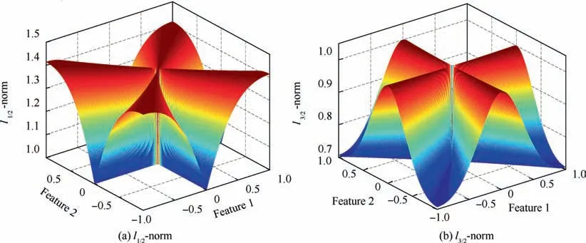
Fig. 1 l1/2 -norm and l3/2 -norm of a two-dimensional vector.

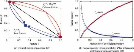
Fig. 2 Optimal sketch and sparse representation of proposed ICF.

Fig.3 Flowchart of proposed intelligent fault diagnosis method.

To investigate the filtering performance of the weights trained by ICF and SF, the weight vectors and their corresponding spectra are plotted in Fig. 6. It can be seen that the weight vectors of ICF with the largest amplitude show narrow spectral bandwidth,and obvious features exist in the frequency domain. However, the frequency components of weights trained by SF are cluttered. The vectors corresponding to features with small amplitude are displayed in Fig. 6(b). The weights of ICF are similar to low-frequency signals, which indicates that features extracted by ICF are not meaningful in this case. As we all know, the weight vector is similar to a filter. Therefore, it also shows that the weights of ICF will not extract any features unrelated to the fault characteristic.Another advantage of ICF is that it shows strong filtering performance when there are other disturbing components in the tested signal.We use different percentages of the fault samples listed in Table 1 for training and the rest samples for testing with the cases ofNin= 100,Nout= 50,Ns= 100 and λ = 1.In order to reduce the influence of the randomness, 20 trials are carried out for each experiment in the following studies.The diagnostic accuracy and time are averaged by 20 trials and the error bars show the standard deviations(the computational platform is a PC with an Intel I7 CPU and 8 GB RAM).The diagnostic results trained by different percentages of samples are shown in Fig. 7 with different training sample numbers.It can be seen that the proposed ICF shows stronger robustness and higher efficiency under the same parameter setting and iteration steps. Therefore, the feature amplitudes extracted by these weight vectors are very small,which ensures the sparsity of features.

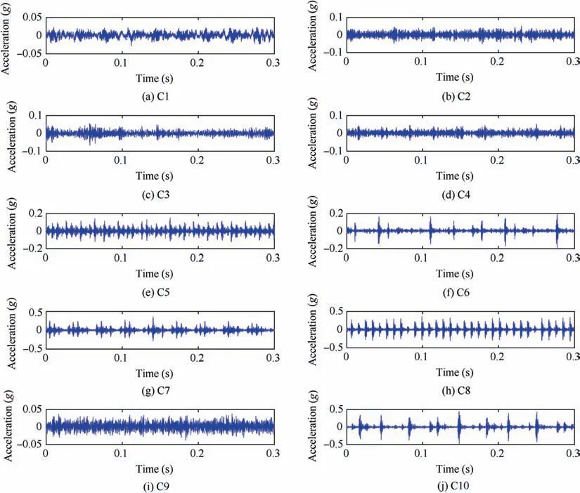
Fig. 4 Description of bearing fault signals.

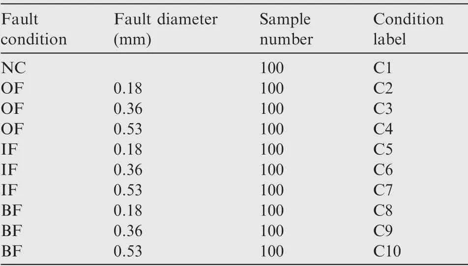
Table 1 Description of bearing fault conditions.

5. Weak signature detection using ICF

In this section,effectiveness of the proposed ICF for impulsive signature enhancement is demonstrated using the simulated and experimental bearing fault data.

5.1. Simulated study

The bearing outer-race failure can be simulated as

whereAis the amplitude coefficient, andB（t） simulates the amplitude modulation component due to the transmission error.Sb（t）, expressed as Eq. (11), represents the periodic impulse component.Tbrepresents the time between two impulse components, which means that the frequency of the shock is 1/Tb. δTdenotes the random jitter caused by the slip effect of rolling elements.frin Eq.(10)and Eq.(11)means the resonant frequency excited by mechanical defects,and α is the attenuation rate of the impulse component.n（t） is the Gaussian noise component to simulate random interference. The definition of signal to noise ratio SNR is shown as follows:

wherePsignalis the power of the signal andPnoiseis the power of noise.Parameter setting of the simulated signals in this section is displayed in Table 2.

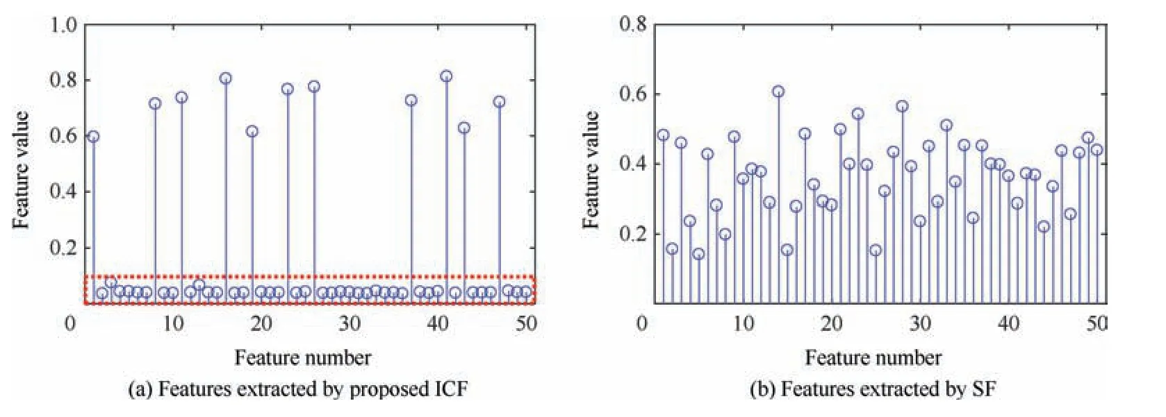
Fig. 5 Comparison of feature distribution (population sparsity) extracted by different methods.

Fig. 6 Weight vectors of roller fault with different amplitudes.

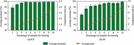
Fig. 7 Diagnostic results using various methods.

The flowchart of the diagnosis method is presented in Fig. 8, and the main steps are summarized as follows:

Step 1.Determine the number and length of filters:NoutandL.

Step 2.Construct the Hankel matrix H ∈RL×（N-L+1）of the sample.

Step 3.Random assignment weight matrix W.

Step 4.Obtain the sample features following the activation function Eq. (3).

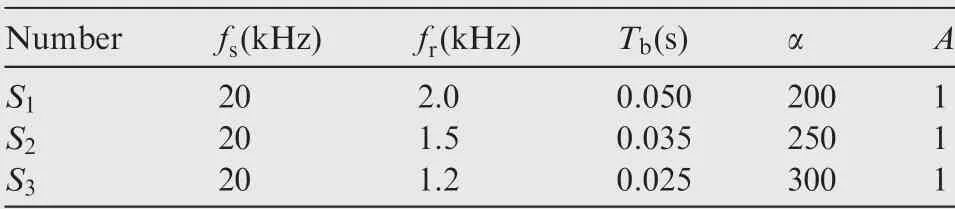
Table 2 Parameter of simulated signals.

Step 5.Calculate the gradient according to the objective function and gradient function, and update the weight matrix through the L-BFGS method.

Step 6.Repeat Steps 4 and 5 until the specified number of iteration steps is reached.

Step 7.Select the optimum filter corresponding to the maximum value of the feature.

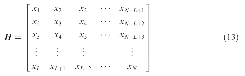
Fig. 8 Flowchart of proposed method for weak signature detection.

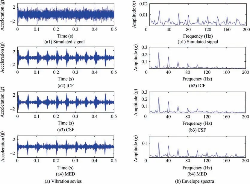
Fig. 9 Diagnostic results of simulated bearing outer-race fault with SNR=-10dB.

In this experiment,Nout= 10, λ = 1,L= 200. The weight vector corresponding to the feature with the largest value is selected as the filter. The detect results using ICF, CSF and MED and the corresponding envelope spectra are plotted in Fig. 9 with SNR = -10dB and Fig. 10 with SNR = -15dB. The results show that the proposed ICF can achieve comparable impulsive signature enhancement performance with CSF and MED when SNR = -10dB. The fault feature can be extracted from the original signal, which can help us to further analyze the fault information through the characteristic frequency and resonance frequency. However, when SNR = -15dB, only the proposed ICF can successfully extract the impulsive component in time domain,which indicates that the weak fault signature can be successfully recovered using the proposed ICF from heavy background noise.

In order to study the effectiveness of the proposed ICF for multi-input systems,S1,S2andS3are simultaneously trained as input samples with SNR = -10dB. In this experiment,in order to improve the training efficiency, the input matrix is constructed by the segments matrix as described in previous section. The training time of the filter is 0.78 s. As shown in Fig. 11, ICF can simultaneously process multiple sets of data with different fault types,which gives us the possibility of handling big data sets.In order to study the robustness of the proposed algorithm,50 experiments were repeated to evaluate the robustness of the algorithm. Fig. 12 shows the robustness for simulated bearing fault signals with different values of SNR.It can be seen that the robustness of the algorithms can achieve 100% whenSNR > -6dB. When SNR = -9dB, the success rate of ICF is still 100%, while CSF and MED are only 68% and 80%, respectively. This shows that the robustness of the ICF algorithm can still be guaranteed in strong noisy environments. When SNR = -12dB, the success rate of ICF is 64%. However, the success rates of CSF and MED are very low,and it is difficult to identify the fault information using CSF and MED.

Fig. 10 Diagnostic results of simulation bearing outer-race failure with SNR = -15dB.

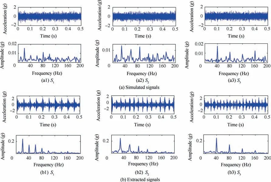
Fig. 11 Results of simulative study for bearing outer-race failure for multi-input system.

Fig. 12 Comparison results of robustness.

5.2. Experimental study

The performance of the proposed method is further validated on an experimental bearing fault dataset. In this experiment,NJ208EM cylinder rolling bearing with outer-race fault was studied. The vibration data were sampled at 25.6 kHz.Throughout this experiment, the bearing is driven by a motor and the rotating speed is kept at 1500 r/min. The detection results using different methods are studied and presented in Fig.13.Through the original time-domain signal and envelope spectrum,we cannot judge the existence of fault due to the fact that there is no obvious fault-related information. ICF and MED separated the impulse component from the original signal using the training filter, which means mechanical damage of the bearing. However, it can be seen from the filtered time-domain signal and envelope spectrum that CSF does not effectively separate the fault components. In addition,although the envelope spectrum of fault signals extracted by MED and ICF is close, the fault components extracted by ICF recover better in time domain,which can help us to study the characteristics of fault in time domain.Consistent with the simulation results, the proposed method performs more superior in impulsive signature enhancement.

Fig. 13 Diagnostic results of different methods for bearings with outer-race fault.

6. Compound fault diagnosis using ICF

In this section, the simulated compound fault signals with noise are utilized to demonstrate the performance of the proposed method for compound fault separation consisting of two shock signals with different fault frequencies and resonance frequencies. Simulated signals in this section are the compound fault displayed in Table 2,S2andS3. The output dimension of ICF is 50, λ = 1,L= 200 and SNR = -10dB. We choose the weights with different frequency components as the final filters. The separated fault components are shown in Fig.14 and Fig.15.We can successfully detect the different bearing faults from the envelope spectrum of filtered components extracted by ICF.The peak values are obvious at the fault characteristic frequency(40 and 33 Hz)and its harmonics,which indicates that an outer-race fault has occurred.In addition, ICF recovers the impulsive signature of the input signal successfully in the time domain. The column constraints of feature matrix trained by ICF require that the distribution of features among different weights is sparse.ICF forces feature peaks between different weights to be generated in different columns to ensure the best sparsity of each column. However, CSF can only extract one component as shown in Fig. 15. It is difficult to identify another fault through the filtered time-domain signal and envelope spectrum.

In this section, the simulated compound fault signals with noise are utilized to demonstrate the performance of the proposed method for compound fault separation consisting of two shock signals with different fault frequencies and resonance frequencies. Simulated signals in this section are the compound fault displayed in Table 2,S2andS3. The output dimension of ICF is 50, λ = 1,L= 200 and SNR=-10dB.We choose the weights with different frequency components as the final filters. The separated fault components are shown in Fig.14 and Fig.15.We can successfully detect the different bearing faults from the envelope spectrum of filtered components extracted by ICF. The peak values are obvious at the fault characteristic frequency (40 and 33 Hz) and its harmonics, which indicates that an outer-race fault has occurred. In addition,ICF recover the impulsive signature of the input signal successfully in the time domain.The column constraints of feature matrix trained by ICF require that the distribution of features among different weights is sparse. ICF forces feature peaks between different weights to be generated in different columns to ensure the best sparsity of each column. However,CSF can only extract one component as shown in Fig.15.It is difficult to identify another fault through the filtered timedomain signal and envelope spectrum.

Fig. 14 Diagnostic results of compound fault using ICF.

Fig. 15 Diagnostic results of compound fault using CSF.

The filter lengthLand output dimensionNoutof ICF are the important parameters that have to be chosen appropriately. The sampling rate, the duration of the signal and the concerned fault frequencies have to be considered when choosing appropriate parameters. In practice, the optimal choice ofLandNoutis not an easy task to find. However, it is found in practice that the proposed ICF is more robust than the CSF and MED filter. The filtering result seems less affected by the choice of filter length.From the authors’experience,a filter length withL= 100 is recommended for initial trials,since this filter length can give satisfactory result for many situations as shown in the case studies.A higherNoutcan obtain more accurate results. However, the calculation efficiency will be reduced. According to the authors’ experience, when the output dimension is less than 5, the robustness is very poor.Therefore, whenNout= 10, the different faults can be separated with strong robustness.

7. Conclusions

This paper proposes a novel unsupervised learning method named intrinsic component filtering for rotating machinery fault diagnosis. The proposed method is validated by the simulated and experimental bearing fault dataset in noise environment. Through the case studies, we can draw the following conclusions. First, the proposed method can adaptively learn various intrinsic features from input samples and achieve comparable performance with SF in terms of intelligent fault diagnosis. Second, compared with the existing methods, ICF performs superior in weak signature detection especially for the multi-input system, which gives us the possibility of handling big data sets. Third, ICF can separate different fault components from compound fault signal without any prior experience.

The limitations of the proposed method and the future research work include the following aspects.First,training efficiency needs to be improved to achieve real-time health monitoring in the application of weak signature detection.Second, the output dimension should be reduced to improve the efficiency and an intelligent feature selection method could be proposed for the separating process in compound fault separation. Third, based on ICF, an intelligent unlabeled compound fault diagnosis method in heavy noisy environment could be studied further for the real-world application. Based on this,the researchers will conduct a detailed study,as well as the improvement and new application of the algorithm.

Declaration of Competing Interest

The authors declare that they have no known competing financial interests or personal relationships that could have appeared to influence the work reported in this paper.

Acknowledgements

The research was supported by the Major National Science and Technology Projects (No. 2017-IV-0008-0045), the National Natural Science Foundation of China (Nos.51675262 and 51975276), the Advance Research Field Fund Project of China (No. 61400040304), and the National Key Research and Development Program of China (No.2018YFB2003300).