Reliability assessment of engine electronic controllers based on Bayesian deep learning and cloud computing
2021-03-16YujiaWANGRuiKANGYingCHEN
Yujia WANG, Rui KANG, Ying CHEN
School of Reliability and Systems Engineering, Beihang University, Beijing 100083, China
KEYWORDS Engine electronic controllers;Cloud computing;Bayesian deep learning;Uncertainty;Reliability assessment
Abstract The reliability of an Engine Electronic Controller (EEC) attracts attention, which has a critical impact on aircraft engine safety. Reliability assessment is an important part of the design phase. However, the complex composition of EEC and the characteristic of the Phased-Mission System(PMS)lead to the difficulty of assessment.This paper puts forward an advanced approach,considering the complex products and uncertain mission profiles to evaluate the Mean Time Between Failures (MTBF) in the design phase. The failure mechanisms of complex components are deduced by Bayesian Deep Learning (BDL) intelligent algorithm. And copious samples of reliability simulation are solved by cloud computing technology.Based on the result of BDL and cloud computing,simulations are conducted with the Physics of Failure(PoF)theory and Failure Behavior Model (FBM). This reliability assessment approach can evaluate MTBF of electronic products without reference to physical tests. Finally, an EEC is applied to verify the effectiveness and accuracy of the method.
1. Introduction
The Engine Electronic Controller (EEC) is a microcomputer with complex design features that controls aircraft engines and affects flight quality and safety.1,2So,the reliability assessment of EEC plays an important role in the reliability design of aircraft. Moreover, the prediction of the most frequently used reliability index in engineering, Mean Time Between Failures(MTBF), has high potential to reduce the development and material cost and testing time, thus saving the cost of aircraft eventually.3,4However,there are two challenges that influence the development of reliability assessment work at the design phase. The first challenge is the complex composition of EEC which leads to the complex process of failure. A regular EEC contains power modules,AC-DC convert modules,signal processing modules,CPU modules,and so on.Each module is regarded as a system composed of a large quantity of electronic components, which causes the difficulty to model the reliability assessment. The second one is the uncertainty in EEC which is caused by external and internal factors. The external factor is that the EEC in the aircraft is a typical Phased-Mission System (PMS). The mission profiles of the EEC change depending on the different mission phases that the aircraft carries out, and it is difficult to evaluate the reliability in the condition that the environment loading is uncertain. The internal factor is that actual products are different from the design because of errors in the production process and measured material parameters. Overall, it is necessary and critical to develop approaches to evaluate the reliability of EEC.
Traditional reliability assessment methods include Markov models, covariate models, and stochastic process models. The Markov model is implemented as an important approach of reliability assessment. Typical examples using the Markov model to evaluate reliability were provided by Liu,5Li,6Guo,7Montoro,8and Dhople9et al. As is well-known, the Markov method has a computational explosion when a complex system model like the EEC is constructed.10In order to solve the problem, some researchers have improved the Markov model. Chen et al.11presented a hierarchical Markov model that can balance the accuracy and complexity of the model. Son et al.12proposed an approach which can decrease the number of states by building Markov models of the independent subsystems stage by stage.The covariate models from reliability prediction handbooks can reflect the factors that affect the failure of electronics.This method is used to attempt to solve the difficulty of reliability assessment due to environmental factors’ uncertainty. Tu13and Xu14et al. used the covariate model to predict the component-level failure rate in order to evaluate the reliability of control strategies and modular multilevel converter. Most of the failures of electronic products are caused by degradation, so in addition to the above models, researchers also use stochastic process models to predict production lifetime. The statistical-based stochastic process models do not need to establish a model to describe the failure process,thus avoiding the modeling problem caused by the complex structure of the EEC. Xu et al.15proposed a hybrid degradation model by combining multiscale characteristic analysis with a modified Gaussian model which predicts the remaining useful life. Li et al.16used a Wiener-process model to predict the remaining useful lifetime of electronics.Whether it is a Markov model,a covariate model,or a stochastic process model, the most important point of using these methods is the fault-related data obtained from the physical test. However, it is difficult to collect EEC data in each phase of mission profiles, which makes these approaches difficult to use. The unique characteristics of the EEC will inevitably require innovative requirements for traditional reliability assessment methods.
The physics of failure approach emerges as an electronic product reliability assessment method that can reflect the impact of failure mechanisms on lifetime. Statistical model and failure database method are based on historical failure rate data,17while the Physics of Failure (PoF) model can predict lifetime using models of failure mechanisms obtained by physics theory. In recent years, more and more electronic reliability assessment studies have been conducted based on the theory of PoF. Sun et al.18used the PoF models to predict the failure rate distribution of an electrolytic capacitor of LED driver systems.Gupta et al19assessed the health monitoring of an Aluminum Electrolytic Capacitor using a degradation model based on PoF. Typical examples using this approach are also included in the research of Zeng20, Temsamani21, and Ren22et al.
Failure Mode and Effects Analysis (FMEA) and Failure Modes, Mechanisms and Effects Analysis (FMMEA) are effective methods for analyzing the failure mechanisms.23,24Trapanese et al.25used the FMEA method to help enhance the reliability of a wave energy conversion system. However,there is a difficulty,which is that failure mechanisms of a complex system are unclear,leading to the inability to select a suitable PoF model to describe the failure process of the product when one solves the reliability assessment problem of a complex system. In order to solve this problem, Lee26used Bayes belief networks in FMEA, and Gargama and Chaturvedi27used fuzzy logic to build the intelligent inference engine for FMEA. With the development of machine learning, the more accurate intelligent FMEA method was proposed by Zhou et al.28FMMEA is a more direct method for analyzing potential faulty machines than FMEA,so intelligent FMMEA analysis method is used to solve analytical difficulties and timeconsuming problems. Bayesian Deep Learning (BDL) as an intelligence algorithm can give the reasoning results in a condition of uncertain information,which combines the advantages of Bayesian network and neural network algorithm.29Ghaisani et al.30has ever used the BDL in the complex and cognitively incomplete medical field to predict the cancer incidence and obtained a prominent accuracy, which indicates indirectly that the BDL algorithm can effectively do the complex inference with uncertainty. Therefore, in this paper, an FMMEA method based on BDL was put forward to solve the failure mechanisms inference problem.
A large amount of computation was required when PoF models were used to evaluate the reliability of a complex system. The EEC contains a large variety of components, and each component is affected by multiple stresses and failure mechanisms at the same time,which requires multiple physical models of faults to be calculated simultaneously for each component.In addition,for PMS,the stress levels at each stage are inconsistent, which requires stress simulation calculations at various stress values. With the characteristics of automated deployment and virtualized computing resources, cloud computing technology has great advantages in dealing with complex computational problems. Jermaina31, Richman32, and Gupte et al.33presented examples where cloud computing technology was used to speed up the simulation process to solve complex simulation problems.
In this paper, an advanced reliability assessment method based on BDL and cloud computing is proposed to improve the EEC reliability. The remaining part of this paper is organized as follows: In Section 2, the process of the reliability assessment methodology is introduced. Section 3 discusses realizing the process of the BDL algorithm. In Section 4, considering the internal and external uncertainty of EEC,reliability assessment based on the cloud computing framework is introduced. Then, a case study and further discussion are presented in Section 5. Section 6 concludes this work finally.
2. Methodology
The reliability assessment approach uses analysis results of failure mechanisms to build PoF models and Failure Behavior Model (FBM) of products to describe the failure. These models considering internal and external cause uncertainty of products are used to estimate MTBF rather than test data.Internal cause parameters contain material parameters, structure parameters and so on. External cause parameters depend on environmental stress and mission profiles.
The procedure of improved reliability assessment methodology is shown in Fig.1. The first step is to confirm all failure mechanisms of each component. Environment and work profiles determine what kinds of failure mechanisms will occur.And failure mechanisms will be obtained by the results of the products’ FMMEA. Hence, the integrality and veracity of FMMEA are important.
The second step is to generate simulation experiment samples considering uncertainty. Product material and structure parameters are dispersive due to material inhomogeneity and machining error. There are uncertain external environmental factors in the working process of electronic products, which are reflected in the mission profiles. These uncertain environment factors will be quantified by extending mission profiles randomly.The result of combining and extending as input profile will be input into reliability simulation.
The next step is the stress simulation using cloud computing.In the methodology, simulation analysis considers the uncertainty in the work process and the reality of work conditions,which makes the simulation object more complex. The more complex the simulation object, the higher the requirements on the computation.Therefore,stress simulations using cloud computing dominate compared with classical simulations with PC.
The final step is to do reliability simulation of components and systems based on PoF theory and FBM,which is an effective approach to do the reliability assessment.In the work process,many failure mechanisms of one component will occur at the same time, which may cause the same type of damage. By calculating the cumulative amount of damage, we can obtain the MTBF, reliability and weakness of the product.

Fig. 1 Procedure of reliability assessment methodology.
3. Intelligent inference of failure mechanisms
3.1. Bayesian inference
The inference result of failure mechanisms is given by the probability of the underlying node of a Bayesian network,and the prior probability table of Bayesian network nodes is given by the neural network algorithm.The Bayesian network is a kind of directed acyclic graph. It can be used for the expression and reasoning of uncertain knowledge. The Bayesian network contains the node information, qualitative and quantitative information of the influence relationship between parent nodes and child nodes.
The connection relationship of evidence nodes of inference logic is described using the two-axis matrix:

wherekrepresents the total of network nodes. ~cijrepresents the connection relationship between nodeiand nodej. If it is one,it means connected.If it is zero,it means no connection.The conditional probability of nodeXiin the network can be passed through

where πirepresents a value set of all parent nodes ofXi,andpirepresents a conditional probability distribution table of nodeXi.From this,we can calculate the probability of failure mechanism under the given environment and product information.
The failure mechanisms are reasoned by calculating the conditional probability of the logical node of the underlying reasoning result under the condition of evidence. To achieve fast and accurate reasoning, junction tree algorithm was used for probabilistic reasoning. The process of building the junction tree is:
(1) Construct a Moral map representing the original Directed Acyclic Graphs (DAGs) of the Bayesian network.
(2) Triangulate Moral map.
(3) Construct a cluster of junction trees.
(4) Establish a joint tree.
After the junction tree is established, the probability distribution table of the corresponding cluster can be changed according to the new evidence, and the reasoning of the Bayesian network is completed through information transmission.The directly connected clusters in the junction tree share a separate node, which contains random variables in these clusters.For example, if a separate nodeZijis composed of two adjacent clustersCiandCj, thenZijcan be expressed as

The separation node contains probability information of the corresponding cluster, and the information propagation between the clusters is bidirectional.The information propagation process involved two probability transformations that are marginalization and combination,and the joint tree algorithm relied on these two changes for probability transfer.LetSiandSjbe two variable sets so thatSi⊆Sj.φjis used to indicate the probability of occurrence ofSj, and the marginalization of φjtoSiis calculated by


where the symbol ‘‘⊗”represents multiplying the mappings of each value of the two functions over the domain.
3.2. Bayesian network parameter estimation
The conditional probability of Bayesian network nodes is corrected by learning data of past failure mechanisms diagnosis.However, it is often the case that the data of past fault mechanisms diagnosis misses some information. In order to learn under the condition of missing information, the expectationmaximization algorithm is used.
The main idea of the EM algorithm is to determine the maximum likelihood estimate of the unknown parameters by maximizing the marginal likelihood of the observed data.The statistical data selected for the training sample is divided into three parts: the first is the observation data setXof the complete information, the second is the unobserved setZof implicit variables, and the third is the unknown parameter ξ.In the independent training sample setaccording to the EM algorithm idea, for the implicit variablezmakesP(x,z) maximum,P(x,z) has a log-likelihood function.

Because there is an implicit variable,l(ξ)cannot be directly optimized.The method was used to continuously establish the lower bound ofl(ξ),called the E step,and then iteratively optimize the lower bound,called the M step,and replacel(ξ)with the optimal lower bound. The lower bound ofl(ξ) can be obtained from Eq. (6) using Jensen’s inequality:

whereQirepresents a certain distribution of the implicit variablez. AndQican be obtained by

Then the pseudo-code of the algorithm is shown in Table 1.
The top-level nodes without parent nodes in the Bayesian network have a direct influence on the trend of the inference process, so the probability of node plays a dominant role in the factors affecting the reasoning results. In order to weaken the human influence in the process of determining the probability of such top-level nodes, the neural network algorithm is used to correct the node prior probability of the top-level node in the Bayesian network. The neurons in each layer of the neural network have a certain influence on the result.The weight coefficient of the neuron contains the corresponding degree of influence information. Therefore, the weight coefficient of each layer of the neural network is used to calculate the absolute influence coefficient, instead of the prior probability of the top-level nodes.The calculation of the absolute influence coefficientEijis as follows:


Table 1 EM algorithm.
whereiis the input unit of the neural network,jis the output unit of the neural network,kis the hidden layer unit of the neural network,Wkiis the weight coefficient between the input layer neuroniand the hidden layer neuronk, andWjkis the weight coefficient between the hidden layer neuronkand the output layer neuronsj.
4. System reliability assessment based on cloud computing framework computing
4.1. Sampling method of uncertainty
The parameters of components in products and the mission profiles have the uncertainty.Even if the model of components is the same, the material parameters and structure dimension parameters will be different because of machining accuracy and impurity in the material.An electronic controller can perform a wide variety of missions,and the types and numbers of missions performed vary throughout its life cycle, so the mission profile is uncertain.In order to describe the uncertainty of electric products, mission profile extending, and Monte Carlo method are used.
As Fig. 2 shows, possibility distributions are assumed for the uncertainty of the material parameter and structure dimension.Each internal parameter of one simulation sample is sampled by the method of Monte Carlo random sampling. These internal paraments and 3D files constitute a complete simulation product. The mission profile consists of basic missions with different ratios, and the seasons and regions influence the environmental stress of the mission profile. Therefore,the number of samples of the mission profileNtpdepends on the number of the kind of basic missions,seasons and regions,which can be calculated by

wherevis the number of regions,miis the number of the kinds of basic missions in theith region,andis the combinatorial number. The number of missions in each sample is given by

whereb1,b2,...,bmiis the ratio of basic missions which reflects the likelihood that the actual task will be performed,tjis each basic mission duration, andTis the specified MTBF of the product design specification.Everymissions are regarded as a minimum mission combination, and thenNtmissions are divided intocombinations with a season in order.The simulation samples generated by this method reflect the uncertainty of products and the mission profiles.
4.2. Failure behavior simulation
The prominent failure mechanisms in electronic components contain cracking of solder joints and components, corrosion of package and lead, electromigration, time-dependent gate oxide breakdown and so on. And gate oxide breakdown and electromigration are related to electrical stress. Thermal cycling and vibration are the major cause of cracking which introduced cyclic stress leading to the failure, and moisture or corrosive substance causes the corrosion mainly at the package and lead. For a review of common PoF models, readers can refer to Refs.34,35
Crack damage caused by different mechanisms has an additive effect. The influence of thermal cycling on the cracking is given by

where TF denotes the number of thermal cycles to failure depending on the high-temperature durationtd, the length of the componentLD, the coefficient of thermal expansion of component and PCB αcand αs, the high temperature of component and PCBTcandTs, non-working temperatureT0and the height of the solderh.CandFare the correction factors which are related to the kind of package and component,and ξfis fatigue toughness factor.

Fig. 2 Process of simulation samples generation.
The influence of vibration on the cracking is given by

where VF denotes the number of vibration cycles to failure depending on inherent frequencyfn, the thickness of PCBH,the ratio of the center of the component to the length and width of the PCBxandy, and output power spectral density at natural frequency pointsPo.Cis the correction factor which is related to the kind of package, andBis the length of the PCB edge parallel to the long side of the component.
Failure time is decided by the speed of damage accumulation. Damage calculation is to clarify the failure time of the sample, and the length of time when the damage reaches the threshold determines the failure time of the system. The amount of damage δ is the degree of damage caused by a mechanism in the product’s working time, and is expressed as

wheretis the time of working andTtis the lifetime obtained from the above PoF models of the mechanism. Each fault physical model of each component can calculate a damage amount, and the cumulative damage calculated in multi-state and phased-mission systems obeys cumulative damage theory as Eq. shows.

whereDis the total amount of damage,ti,jis the working time of thejth stage of theith mission,is damage factor indicat-ing the degree of interaction between the failure mechanism FMqand other mechanisms,is the unit amount of damage caused by FMqandis the unit damage index of FMq. The simulation time when the damage amount reaches the damage threshold is considered as the failure time.
When the same component has multiple failure mechanisms at the same time, there are multiple damages. The length of time corresponding to the damage amount that reaches the damage threshold ω is the failure time of the componentTec.

Electronic product failure timeTpis given by

Each simulation sample can obtain the damage amount of the sample and the failure time of the sample under the design lifetime.The production of each sample is equally possible andfT(t)is the probability density function of the time between failures, so the MTBF assessment of the product is the expectation ofTp.

4.3. Cloud computing framework of simulation
The automatic simulation process is presented in the article to eliminate the need to manually set the next simulation parameter at the end of each simulation. The automatic simulation method is required for stress simulation based on cloud computing technology because it can make the parameters of a great deal of simulation samples be automatically set. Here,taking the random vibration simulation as an example, the simulation automation process solution is given in Fig. 3.
As Fig. 3 shows, the JAVA language is used to establish ANSYS software interface to read files, and the files are input into ANSYS software to establish three-dimensional model and fixed constraints. The APDL language is used to apply random vibration loads on the ANSYS simulation model.After the simulation input is completed, ANSYS software is used to perform modal analysis and random vibration analysis in sequence. For modal analysis, first, the three-dimensional model is meshed. Then, fixed constraints are applied to the meshed three-dimensional model. Finally, finite element analysis is performed (final treatment). The three-dimensional model with fixed constraints and the grid is also used as the input condition of random vibration simulation, and the simulation is carried out after applying the random vibration loads.Finally,colored stress patterns,vibration attribute value and simulation log files are obtained from the software output files.
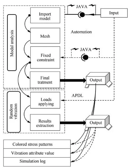
Fig. 3 Automatic simulation process solution of random vibration.
As it is demonstrated in Fig. 4, user data is transmitted to the cloud computing core through the client data channel and cloud data access port.The cloud computing core simultaneously calculates vibration simulation, thermal simulation,and damage accumulation calculation. The computing cores of the cloud are combined with database information for thermal simulation, vibration simulation, and durability simulation.Finally,the calculation results are transmitted to the user via the cloud data access port.
5. Case study
5.1. Structure of engine electronic controller
The main function of the electronic controller is to receive the measurement signal of the sensor and output a control signal to the actuator after performing a series of processing inside the signal. The structure of the electronic controller is shown in Fig. 5.
The electronic controller can be divided into three modules:the input signal conditioning circuit, the core CPU and the output signal conditioning circuit. The input signal conditioning circuit is subdivided into analog input conditioning module, frequency input conditioning module and digital input conditioning module according to different types of signals received by CPU. The output signal conditioning circuit is divided into analog output driving circuit and digital output conditioning circuit. And the power module supplies power to the above modules. The control logic structure of the core CPU is Min-Max structure. The Min-Max structure is composed of several transient control loops as well as a steadystate control loop, each responsible for providing one of the requirements or provisions of the engine. Fig. 6 shows Min-Max structure for the controller presented in the CPU. The transient control loops are to protect the engine against limiting constraints, including maximum speeds of power turbine shaft (NPT) and gas generator turbine shaft (NGG), required NPT, maximum acceleration, and maximum negative acceleration (deceleration). The steady-state control loop is responsible for providing enough fuel for the engine’s steady-state condition. The signal collected by the sensor from the engine is passed to the CPU for processing through the input signal conditioning circuit. The CPU controls the engine’s fuel input via the output signal adjustment circuit,which in turn controls the engine’s operating state. As hardware structure and software structure are demonstrated, failure of any component in the electronic controller will result in system failure.

Fig. 5 Engine electronic controller.

Fig. 6 Modules included in engine electronic controller.
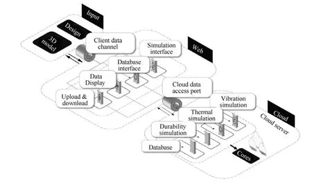
Fig. 4 Stress simulation framework based on cloud computing technology.
5.2. Failure mechanisms inference based on BDL
As for the components in EEC, the initial Bayesian networks were established by using the failure mechanism case. The parameters of the EM algorithm and the neural network algorithm are shown in Table 2.
Taking metal film resistor as an example, according to the extracted fault mechanism reasoning logic relation rules, the results of constructing the Bayesian network by MATLAB are shown in Fig. 7.
Nodes 1-4 represent typical locations where microelectronic devices fail, nodes 5-12 represent the environmental conditions under which the microelectronic devices operate,and nodes 13-18 indicate possible failure mechanisms.The figure uses arrows to indicate the causal relationship between the parent nodes and the child nodes and there is no direct causal relationship between unconnected nodes.
According to the known working environment conditions:humidity, high temperature, vibration, and high voltage or current, the evidence set value of these was one. Except for known working environment conditions, the evidence for the remaining environmental conditions was unknown. The reasoning results are shown in Fig. 8 below. For the correspondence between abbreviations and failure mechanisms, please refer to Appendix A.
5.3. Stress simulation using cloud computing
According to the design requirement of the electronic controller, it takes eight basic missions in all seasons and six regions.So,the number of profile samplesNtp= 1145 according to Eq. (12). And the internal parameters of products obeyed normal distribution. As for mission profiles of PMS,Power Spectral Density(PSD)of the acceleration and temperature profiles of eight basic missions are shown in Figs. 9 and 10. For example, Figs. 9 (a) and 10 (a) represent the temperature and vibration changes experienced by the basic task (a),respectively.
Since the season did not affect the vibration characteristics,the PSD of Fig. 9 did not change with the season. In Fig. 10,the dotted line in each sub-graph represents the temperature change experienced when performing this basic task in the cold season, and the solid line represents the temperature change experienced in the hot season.Simulation projects with 45 temperature simulation points from the lowest temperature to the highest temperature and 70 vibration simulation points were simulated according to the stage of basic missions.
Each simulation sample was subjected to stress finite element simulation and there were multiple stages in the mission profile of the simulation sample.Hence,the copious simulation samples in quantity caused that simulation duration was so long that it could not be accepted.Therefore,if the cloud simulation method was not used for stress simulation, the time cost of the simulation would be unacceptable. Simulations were performed using cloud computing simulation software platform CRAFE which was developed for achieving this method. And parts of the simulation results are shown in Fig.11.The external stress parameters used by the PoF model were extracted from the stress simulation cloud map in order to obtain the product failure time under different tasks and regions.
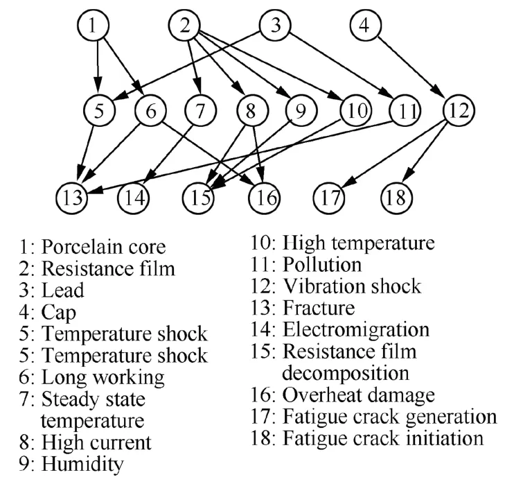
Fig. 7 Bayesian network modeling for metal film resistor.

Table 2 Algorithm parameters.
5.4. Reliability assessment
In Fig. 8, the failure mechanisms of each device were the first two with the highest probability of occurrence. According to the failure mechanisms of the components, PoF models are shown in Table 3.
The stress value at the component position was extracted,and the damage amount of each task phase was calculated using the selected PoF model.The product’s damage threshold was set to 0.8 to estimate the MTBF of the product sample.After statistics, the MTBF values of all samples are shown in Fig. 12.

Fig. 8 Failure mechanisms inference.

Fig. 9 PSD of acceleration of eight basic missions.

Fig. 10 Temperature profiles of eight basic missions.
As can be seen from Fig.12,the life frequency distribution of the product has three main crests, which correspond to the three weak points in the EEC. The Gaussian model and the skew-normal model were used to fit the life distribution data.The form of the Gaussian model is as follows:
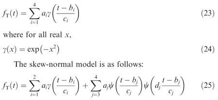
where ψ is the normal distribution function and[ai,bi,ci,di]are the model parameters.
Table 4 demonstrates that the skew-normal model is better than the Gaussian model. And then according to Eq. (22),
Table 5 was obtained by conducting the EEC field tests.Each test corresponded to a basic task condition. After each failure, the EEC was repaired until all basic tasks were completed, and the time of each test and the failure in this period were recorded. This test method is a time-censored test. In GJB899A, the estimation method for the time-censored test is given.The MTBF point estimatefor the time-censored test is as follows:

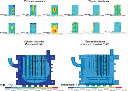
Fig. 11 Thermal and vibration simulation results.
whereTtotalis the total duration of the time-censored test andris the number of faults in the test.Therefore,point estimate of the data in Table 5 is ^θ=3094.75 h.

Fig. 12 MTBF of all samples and some fitted models.
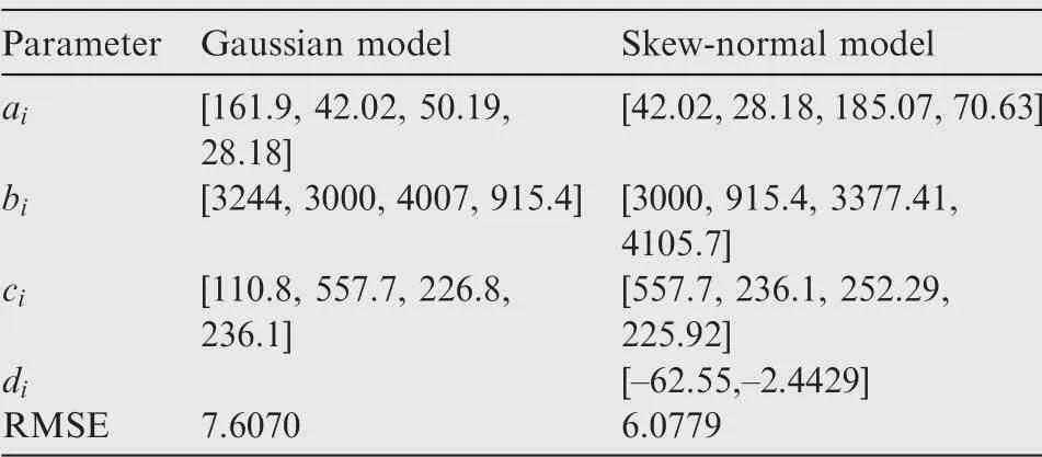
Table 4 Model parameters estimation results.
The one-side lower confidence limit θLof MTBF with confidenceCθ=80% commonly used in practice is

where θL(Cθ,r) is the one-side lower confidence limit coefficient, and can be calculated by

To further illustrate that the current data can support the analysis in the article, hypothesis testing is performed. The MTBF of electronic products of complex systems tends to follow an exponential distribution. If the populationX={X1,X2,···,Xn} of the exponential distribution sample follows the exponential distribution of the parameter η, then MTBFThus the statistic γ = ηfollows the distribu-tion Γ with the parameter (1,η),that is,the probability density functionf(x) of γ is

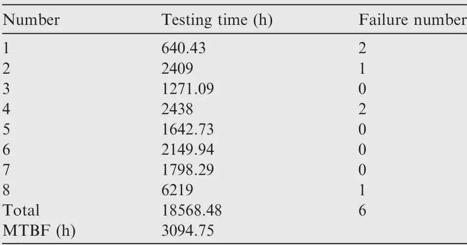
Table 5 MTBF of EEC working for basic missions.
whererepresents the sample mean, andnrepresents the number of samples.
Given a significance level α = 0.05,we test the null hypothesis
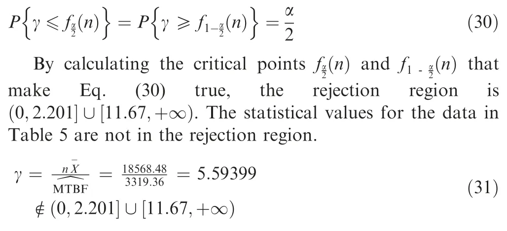
Therefore,the original hypothesis is accepted.Through the above supplementary analysis, it can be concluded that the estimated value ^MTBF obtained by the method proposed in the paper is close to the result obtained by the experimental method. The error between the estimated value ^MTBF and point estimate ^θ is 6.77%, and the error is acceptable. The main source of this error may be other types of fault behaviors besides damage accumulation in EEC,and there may be occasional faults in the actual use of EEC.
When the product failed,the damage amount of the corrosion mechanism is shown in Fig.13(a).Although the corrosion mechanism did not eventually lead to product failure,the damage amount had been close to the threshold.If the product life extension is required, corrosion protection measures will be required for the product. It can be found from Fig. 13(b) that the occurrence of the corrosion mechanism has a strong regional correlation. Therefore, it is necessary to pay attention to corrosion protection during the design.

Fig.13 Corrosion mechanism.
6. Conclusions
(1) Combining BDL with cloud computing, an advanced method considering complex PMS and product uncertainty is proposed to estimate the MTBF of EEC.Compared with the traditional method,this method takes the uncertainty of internal and external causes into account. Moreover,through the case study in Section 5,it can be found that this method can evaluate the MTBF of electronic products without reference to physical tests, so it can be used as a reliability evaluation method in the design stage.
(2) A method based on BDL for FMMEA is proposed to infer the possible failure mechanism. In the case, this method solves the problem of Bayesian network coefficient evaluation caused by insufficient understanding of the failure mechanism of complex PMS products and reduces the dependence of FMMEA on expert experience.
(3) The application method of cloud computing technology in the field of reliability evaluation is proposed,and the cloud platform software CRAFE for reliability evaluation is developed according to the software framework structure proposed in this paper.In the case,cloud computing solves the problem of large amount of simulation calculation when considering the product’s internal and external uncertainties. It improves the feasibility of MTBF evaluation using the reliability evaluation method proposed in this paper.
(4) A certain type of electronic controller is taken as an example for case analysis. The MTBF calculated by the method proposed in this paper is close to the MTBF point estimation value obtained through the analysis of test data and is located at the confidence interval. And the result of hypothesis testing illustrates the effectiveness of the method. Designers can formulate regular maintenance plans based on MTBF. Based on the results of intelligent reasoning of the failure mechanism,the failure mechanism that induces the failure of the simulation sample, and the statistical results of the damage amount of the failure mechanism, the designer can obtain the failure mechanism and key components that ultimately induce the failure, then prevent the failure mechanism in design and design the corresponding Built In Test (BIT) system or Prognostics Health Management (PHM) system for key parts.
Declaration of Competing Interest
The authors declare that they have no known competing financial interests or personal relationships that could have appeared to influence the work reported in this paper.
Acknowledgement
This study was supported by the National Natural Science Foundation of China (Nos. 61503014 and 61573043).
Appendix A.
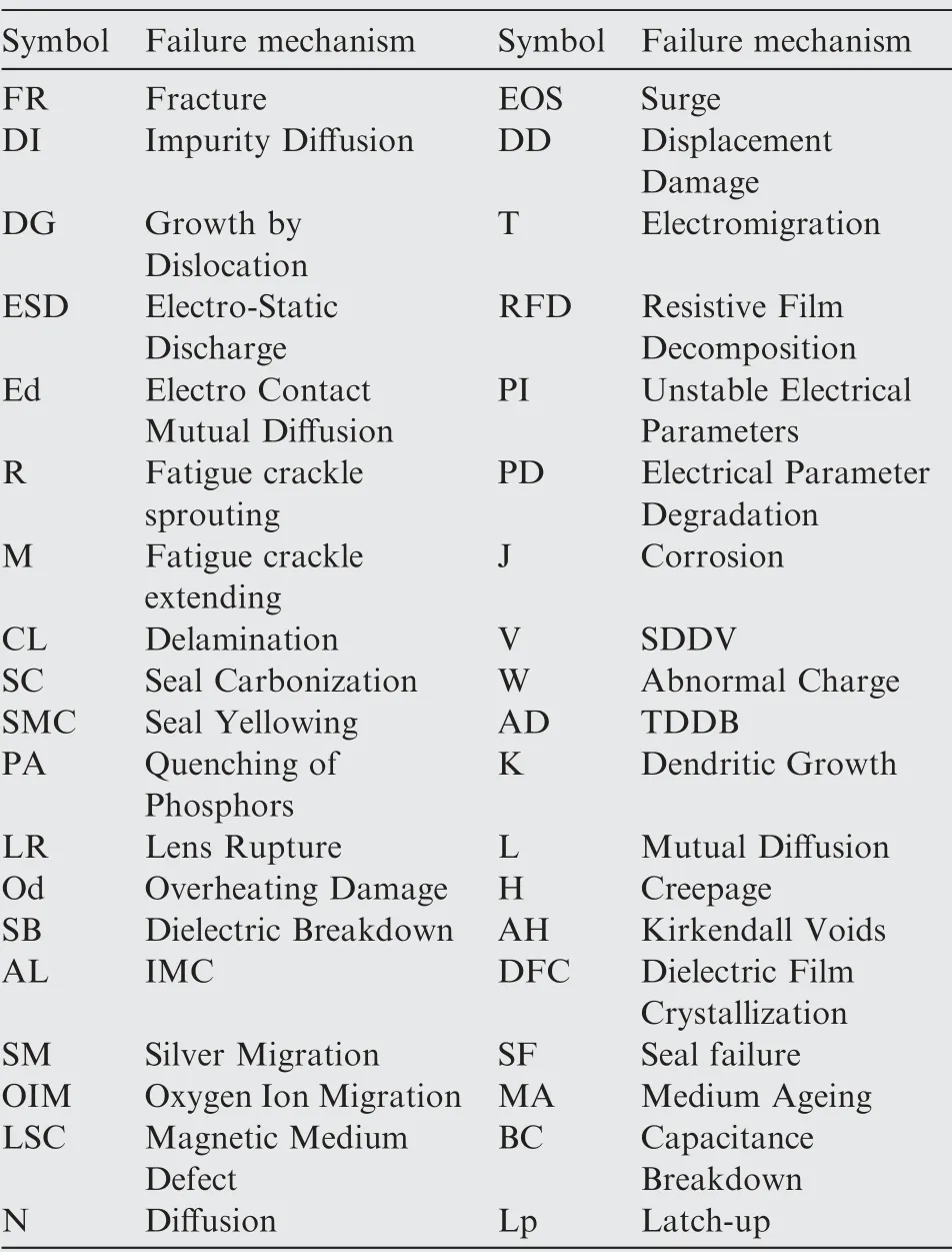
Table A1 Correspondence between abbreviations and failure mechanisms.
杂志排行
CHINESE JOURNAL OF AERONAUTICS的其它文章
- Tangling and instability effect analysis of initial in-plane/out-of-plane angles on electrodynamic tether deployment under gravity gradient
- Aerodynamic periodicity of transient aerodynamic forces of flexible plunging airfoils
- Effects of swirl brake axial arrangement on the leakage performance and rotor stability of labyrinth seals
- Experimental and computational investigation of hybrid formation flight for aerodynamic gain at transonic speed
- Tomography-like flow visualization of a hypersonic inward-turning inlet
- Hypersonic reentry trajectory planning by using hybrid fractional-order particle swarm optimization and gravitational search algorithm
