l1-based calibration of POD-Galerkin models of two-dimensional unsteady flows
2021-03-16RiccardoRUBINIDavideLASAGNAAndreaDARONCH
Riccardo RUBINI, Davide LASAGNA, Andrea DA RONCH
Faculty of Engineering and Physical Sciences, University of Southampton, Southampton SO17 1BJ, United Kingdom
KEYWORDS Computational methods;Dynamical systems;Lid-driven cavity;L1-based regression;Reduced order models;Sparsification;Stabilization of ROMs
Abstract This paper discusses a physics-informed methodology aimed at reconstructing efficiently the fluid state of a system. Herein, the generation of an accurate reduced order model of twodimensional unsteady flows from data leverages on sparsity-promoting statistical learning techniques. The cornerstone of the approach is l1 regularised regression, resulting in sparselyconnected models where only the important quadratic interactions between modes are retained.The original dynamical behaviour is reproduced at low computational costs,as few quadratic interactions need to be evaluated.The approach has two key features.First,interactions are selected systematically as a solution of a convex optimisation problem and no a priori assumptions on the physics of the flow are required.Second,the presence of a regularisation term improves the predictive performance of the original model,generally affected by noise and poor data quality.Test cases are for two-dimensional lid-driven cavity flows, at three values of the Reynolds number for which the motion is chaotic and energy interactions are scattered across the spectrum.It is found that:(A)the sparsification generates models maintaining the original accuracy level but with a lower number of active coefficients; this becomes more pronounced for increasing Reynolds numbers suggesting that extension of these techniques to real-life flow configurations is possible; (B) sparse models maintain a good temporal stability for predictions. The methodology is ready for more complex applications without modifications of the underlying theory, and the integration into a cyberphysical model is feasible.
1. Introduction
Future air and sea vehicles will be self-aware. The concept of self-awareness1requires the ability to monitor the vehicle internal state, to sense the surrounding environment, and to assess its capabilities currently and to project them into the future.This requires integration of multiple individual technologies and development of integrated technologies.2Self-aware vehicles have immediate and future applications, i.e. on-demand mobility, and include the full spectrum of aircraft, from small unmanned vehicles to large transport aircraft. Among the required technologies identified in Ref.1for a self-aware aircraft concept, the present work focuses on the development of physics-informed models of the current system states and the capability to forecast the temporal evolution of the system at low computational costs for on-board, real-time applications. Generally, the development of required technologies for self-aware vehicles is driven by nature, as discussed thoroughly in the review work.2A recent and excellent contribution on bio-inspired concepts and existing flying prototypes is presented in Ref.3.Despite the need to advance a multitude of individual technologies, morphing continues to be one of the most popular research venues.4For example, Ref.5presents a numerical study of morphing wings that are compared to a conventional wing in terms of aerodynamic performance.On a different but complementary subject, Ref.6proposed a novel load prediction tool that extends analytical theories.Predicted loads are parametrised by wing planform geometry,making the tool suitable for exploring a large design space in topology optimisation studies or for predicting the system response (aerodynamics, flight dynamics) when damage characteristics are detected in real-time by sensor networks. The seminal work in Ref.7optimised the external aerodynamic surface of an aircraft over an entire flight trajectory,going beyond state-of-the-art single or multi-point optimisation.The optimisation leverages on morphing technologies that are coordinated with the appropriate stage of the flight path, providing superior performances compared to a fixed wing aircraft.
This paper provides an overview of a recent technology development effort aimed at identifying the aerodynamic/fluid states of a system with no a priori aerodynamic knowledge.The approach is general in its formulation and shall see applications in different fields than those documented herein. To demonstrate the proposed approach,a canonical fluid mechanics problem is used as test case.The extension to a fully threedimensional problem,i.e.flow around a membrane wing,or to a coupled problem, i.e. fluid-structure interaction, is straightforward and entails no modifications to the underlying theory.
Reduced Order Modelling (ROM) techniques have gained significant importance both as analysis and prediction tools.8-11This increase in popularity can be attributed to the availability of large amount of data from experimental and numerical sources.12,13A well-established approach consists in projecting the governing equations onto the subspace spanned by the firstNmodes obtained from a suitable modal decomposition.14,15The choice of the modal decomposition is not unique,15,16but depends upon the aspects of the flow one wants to highlight. One of the most popular choices is Proper Orthogonal Decomposition(POD),mainly for its properties of energetic optimality and the consequent ability of generating compact and parsimonious representations of the original dataset.15,17,18
Galerkin projection of the governing equations onto the POD subspace results in a system of coupled Ordinary Differential Equations (ODEs) with a quadratic nonlinearity described by a third order tensor Q,representing the quadratic interaction between pairs of different modes. Due to the nonlocal nature of the spatial modes and no a priori assumptions on the flow field all entries of Q are generally non-zero. This results in a computational cost scaling asO(N3) for a model constructed withNmodes. Models that include all possible quadratic interactions are referred to as dense or densely connected.
When the Reynolds number grows and the range of energyrelevant spatial scales widens,19a larger number of modes is required to reach a satisfactory energy resolution. As a consequence, a complete evaluation of the nonlinear interactions can quickly become prohibitive.This limits the use of Galerkin models in real life applications, where the number of modes needed to reconstruct a satisfactory amount of kinetic energy might be large. A possible solution is to construct a reduced order model considering only a small amount of modes. If the POD is used this is equivalent to simulate the large scales of the flow and models the smallest ones. Commonly, this approach results in lack of accuracy and temporal stability of the corresponding ROM.9The main problem arising from the truncation process is the elimination of the smallest and less energetic scales of the flow20responsible of the dissipation of the kinetic energy generated at the larger scales. This is a well-studied issue and it is usually tackled with the introduction of a sub-grid dissipation model.9,14A second aspect undermining the accuracy of reduced order models is the lack of quality of the numerical or experimental data the models are generated from. Often times, numerical simulations are not carried out on complete dynamical representations of the flows(sub-grid modelling in large eddy simulations, for example)while experimental results can be corrupted or affected by measurement errors.12The joint effect of truncation of poor data quality can make obtaining accurate short time predictions a challenging task.
This work aims to extend the current literature in term of calibration techniques for reduced order models. Recently,various approaches have been proposed to calibrate and improve the accuracy of the reduced order models.12,21-23They all share the idea of leveraging the knowledge of the true temporal dynamics of the flow in order to adjust the numerical value of the coefficients in the ODEs system through an optimisation procedure.A simple approach consists in performing least squares regression on the system coefficients. This approach can provide satisfactory results in case of small ROMs and good quality data to train the algorithm.In real life configurations,as observed by Refs.12,24,small and poor quality datasets are very common. This makes the use of a pure least squares regression technique without any regularisation term strongly discouraged. Refs.12,25proposed an approach based on a Tikhonov penalisation term to control the numerical values of the coefficients in the reduced order model. This approach is a well established statistical learning technique used to regularise least squares regression problems where the database or feature matrix has poor numerical conditioning.24,26Although the Tikhonov regularisation has been proved successful for relatively small models a possible drawback is that this regularisation preserves in the tuned model all the coefficients present in the original one. Since for POD-based Galerkin models the number of coefficients grows asO(N3), the resulting least squares problem might require a prohibitive number of snapshots to perform a meaningful regression without incurring in overfitting problems. The proposed solution to overcome this limitations exploits the observation that the dynamics of the flow is not equally influenced by all the coefficients contained in Q but, on the contrary, it is mainly governed by a small number of flow structures generating a reduced order model where only a subset of interactions is relevant for the dynamics.27-30Therefore,an algorithm able to automatically identify the subset of relevant interactions could be beneficial to improve the computational performances and facilitate the calibration of ROMs of complex flows.
Work in this direction has been recently done by Brunton et al.31,who developed the SINDy framework to identify equations generated by a system that already possess a sparse structure. A further extension of the SINDy has been proposed by introducing energy preserving constraints to improve the prediction accuracy of POD-based Galerkin models without the need of high-fidelity solver to project the Navier-Stokes equations.32In this paper,the aim is to extend these ideas using thel1sparsity promoting regression to systematically identify the leading coefficients in a priori dense Galerkin systems. To this end, we identify the coefficients associated with the interactions between modal structures that play the dominant role in the dynamics. Once this subset is identified, tuning the numerical values of the coefficients to improve the performances of the model is more convenient. The main advantage of the proposed approach is that only a small subset of coefficients is retained after sparsification and,as a result,the tuning of the coefficients requires a considerably smaller dataset.
The present paper is structured as follows.The first part of Section 2 summarises the methodology utilised to generate Galerkin reduced order models. Subsequently, thel1based regression is outlined and a discussion on how it can be leveraged to generate sparse representation of originally dense models is presented.In Section 3,we demonstrate this approach on a family of large POD-based reduced order models of chaotic solutions of lid-driven cavity flows at different Reynolds numbers for which Direct Numerical Simulation (DNS) is performed. Results are divided into two main sections. In the first,the focus is on the effects of the complexity of the reduced order model on the sparsification.Second,the predictive capabilities of the sparse models are compared with their dense counterparts and with DNS simulations.
2. Methodology
2.1. Galerkin-based reduced order modeling
A modal decomposition represents the fluctuating part of the flow field u′(t,x)=(x)-u(t,x), where the(x) is the mean flow, as a finite sum ofNtemporal and spatial modes as
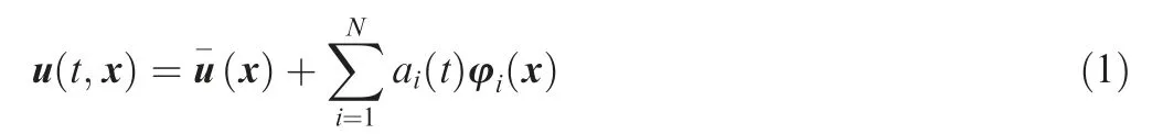
The coefficientsai(t)and φi(x)(i=1,2,...,N)are the temporal and spatial modes, respectively. If the modes form an orthonormal basis of a space Ω where the canonical scalar product is defined as (·,·), the fluctuating kinetic energy is defined as

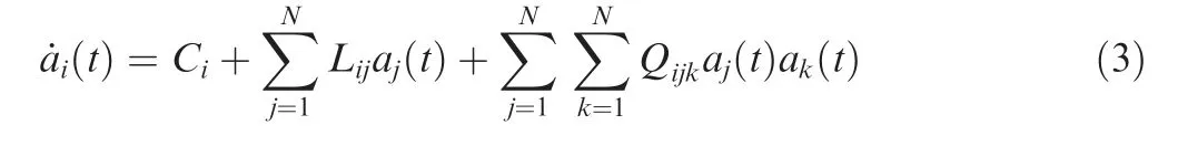
Since the spatial modes incorporate automatically the boundary conditions of the problem, this provides a suitable basis to generate reduced order models of flows in arbitrary geometries.Reduced order models are then derived by projecting the governing equations onto the subspace defined by the firstNmodes. Assuming appropriate boundary conditions14and orthogonality of the spatial modes,this results in a system of coupled nonlinear ODEs defining the temporal evolution of the coefficientsai(t).The tensors of coefficientsCi,LijandQijkare defined in Ref.14and describe the constant, linear and quadratic interactions between modal structures. Here, we focus on the nonlinear interactions term in Eq. (3),Qijkaj(t)ak(t). Without any a priori assumption on the flow physics and on the boundary conditions,due to the global nature of the spatial basis functions φi(x)all entries ofQijkare different from zero.This means that the evaluation of(t)at any instant of time requires the evaluation of all the linear and quadratic interactions between the mode itselfai(t) and the other modesaj(t) withj=1,2,...,N. Due to the mathematical structure, the number of coefficients evaluated at every time step and, consequently, the computational complexity of the model grows with the number of modes asO(N3).
Since we know that flow structures associated toaj(t)ak(t)do not interact in an arbitrary way but some interactions are favoured over others,we assume that not all the entries ofQijkhave the same importance in describing the evolution of ˙ai(t).Therefore, we aim at developing a systematic procedure to enable us identify a sparse tensor,that is a good approximation of the original tensorQijk,in the sense that at any time

The identification of the subset of most relevant interactions is beneficial allowing to reduce the number of active coefficients in Eq. (3) without affecting the accuracy of the system itself. We will refer to this new set of coefficients as sparse or sparsely connected reduced order model.
2.2. Sparse regression
We use sparse regression to identify the most important quadratic interactions inside the set of Eq. (3). AssumingNTsnapshots of the velocity field are available from simulation, we arrange the projectionsai(tj)=withi=1, 2,...,Nandj=1, 2, ...,NT, into the data matrix A ∈RNT×N, where theith column represents the evolution of theith mode, while thejth row contains the state vector at timetj. We exploit the polynomial structure of the Galerkin Eq. (3) to construct the database matrix Θ(A)∈RNT×q.
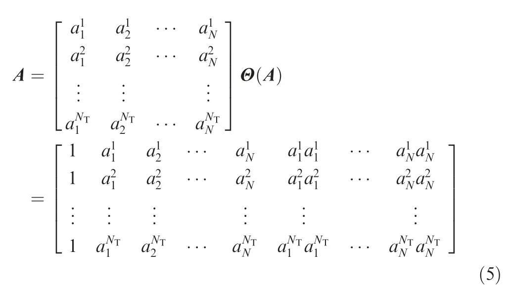
whereq=(N+1)+N(N+1)/2 is the total number of interactions present in the Eq. (3), the sum of constant, linear and quadratic interactions.The number of quadratic coefficients isN(N+1)/2 instead ofN2since the interaction between the modeiandjis considered only once in the definition of Θ(A). This avoids generating columns of Θ(A) that are linearly dependent, which would result in numerical issues in the solution of the regression (see e.g. Perret et al.33). Analogously to what done in the construction of the matrix A, we construct the modal acceleration matrix ˙A ∈RNT×N, containing the time derivative of the temporal coefficients by projecting the modes φi(x) on the corresponding snapshots of the Eulerian acceleration field ∂tu(tj,x). Arranging the coefficients tensorsCi,LijandQijkof theith mode into a vector βi∈Rq,theith Eq. (3) is rewritten as

where the dynamics associated with the mode ˙ai(t)is contained in theith column of the matrix ˙Ai.
The assumption that not all interactions in the nonlinear termQijkajakhave the same importance is equivalent to assuming that some coefficients in βiassociated with the columns of Θ(A)can be set to zero without affecting the value of the corresponding column ˙ai(t).Thus,the idea is to prune some of the entries of βi, corresponding to columns of Θ, by solving the optimisation problem
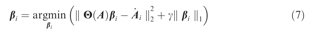
depending on the regularisation weight .This is al1regression problem also known as LASSO (Least Absolute Shrinkage Selection Operator) regression.34It is a well studied convex optimisation problem for which numerous efficient routines have been developed. The objective function in Eq.(7) is composed of two terms. The first is a least-squares term that penalises the distance in modal space between the acceleration of the reconstructed system, the term Θ(A)βi, and the objective ˙Ai. The second term is a penalisation on the regression coefficients weighted by the variable coefficient γ in Eq.(7). It encourages sparsity in the solution shrinking to zero the entries of βithat have the least contribution to the dynamics of ˙ai(t). More specifically, thel1norm is proven to be the best convex approximation of the cardinality operator that counts the nonzero entries of βi.35
After the solution of Eq. (7) is obtained, we define the relative reconstruction error ε as
where the reconstruction error is normalised with respect to the corresponding amplitude in order to balance the error
across the spectrum of modes. We also define the global density as
where the cardinality operator card(βi) counts the number of entries of βidifferent from zero. The cardinality of βican be also defined in term ofl0norm ‖βi‖0providing a formal definition of sparsity of the vector βi. A family of models can be generated by varying the regularisation weight γ. For small weights, dense models with good prediction accuracy are obtained and vice versa for large weights. We can display this family of models on a ρ-ε plane,producing a curve referred to as sparsification or ρ-ε curve. Since only a subset of interactions is relevant, many of the entries ofQijkwill be shrunk to zero when increasing the regularisation weight,without affecting significantly the error ε. This produces a sweet spot in the sparsification curve, defining an ‘‘optimal” value of γ and a consequent optimal value of the model density ρ=ρopt,corresponding to models with low density and low reconstruction error where only the relevant interactions for the flow physics are preserved.
3. Results
In this section this methodology is applied on the two dimensional flow developing inside a lid driven square cavity. First,the flow characteristics and the modal decomposition is presented. Second, the different dense ROMs are generated by Galerkin projection. Lastly, the performance of the sparse models compare with the correspondent dense model and the baseline DNS simulation are analysed.
3.1. Test case and modal decomposition
The Reynolds number is defined asRe=LU/ν,whereLandUare,respectively,the cavity edge and the lid velocity.The kinematic viscosity is denoted by ν. In this work the edge length and the lid velocity are set equal to 1 in non-dimensional units and different values ofReare obtained varying the values of ν.More specifically, three different values of Reynolds numbers are considered. Namely, 1×10⁴, 2×10⁴and 5×10⁴. The dynamics in these conditions is chaotic with increasing complexity for increasing Reynolds number, as shown by Auteri et al.36The domain is defined in nondimensional Cartesian coordinates x=[x,y] and the velocity field is defined by the components u=[u,v]. The simulations are performed in OpenFOAM using a modified version of the solver icoFOAM that also outputs the snapshots of the Eulerian acceleration∂tu(t, x) to compute the modal acceleration ˙ai(t) needed in Eq. (7) more accurately. The convective and viscous terms are spatially discretised with a second order finite volume technique and the temporal term with a semi-implicit Crank-Nicholson scheme.
Fig. 1 shows the vorticity field ω= (∇×u)zat the same time instant for the three Reynolds numbers considered. For the lowest Reynolds number, a strong shear layer separates the main vortex from the recirculation areas in the cavity corners. As the Reynolds number increases, the vortex on the lower right corner is shed and advected by the mean flow along the shear layer. This phenomenon is accompanied by strong,quasi-periodic bursts in the turbulent kinetic energy. For the highest value of Reynolds number, the set of vortices breaks the shear layer while being transported downstream by the mean flow.A preliminary study was carried out to ensure that the average flow quantities reached statistical convergence.This is an important aspect to satisfy to obtain reliable cross-validated results in the regression.To this end,the eigenvalues of the POD decomposition were monitored. It was found that a database of lengtht=100 time units is adequate for the case atRe=1×10⁴, increasing tot=200 time units atRe=2×10⁴, and finally tot=300 time units atRe=5×10⁴.
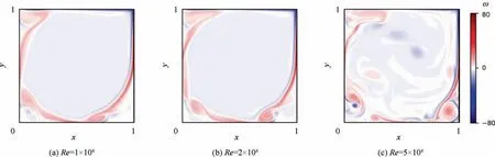
Fig 1 Lid-driven cavity flow: Snapshots of vorticity field for different Reynolds numbers.

Fig. 2 The first 50 eigenvalues of POD decomposition and vorticity fields of the first and most energetic spatial POD mode for three Reynolds number considered.
Fig. 2 (a) reports the first 50 eigenvalues (λi) of the POD decomposition of the three test cases already presented in Fig. 1. It is observed that the eigenvalues increase monotonically for increasing Reynolds number,as turbulent fluctuations contain increasingly more energy. One also observes that, for the two lowest Reynolds numbers, consecutive eigenvalues appear in pairs with similar value. This feature reflects the presence of an unsteady motion in a quasi-periodic regime,characterised by pairs of spatially-similar structures shifted in space, describing the evolution of a wave travelling along the shear layer.Evidence of this feature can be found in Figs.2(b) and (c). Similar structures have already been observed in Ref. 37 for Koopman eigenmodes of cavity flow at similar flow conditions. At the highest Reynolds number, Re=5×10⁴,the flow contains a wider hierarchy of modes. The eigenvalue spectrum (triangles) has a slower decreasing trend, without pairs of adjacent eigenvalues.The most energetic spatial eigenmode in Fig. 2(d) captures the generation and shedding of a vortex on the lower right corner, with no significant activity in the shear layer.This observation is confirmed by inspecting the temporal evolution of the velocity field, revealing the formation of a high energy vortex on the lower right corner transported downstream by the mean flow. First, the temporal correlation matrix between two snapshots defined at two instants of time, ti and tj, defined as S ∈RNT×NT with entries
where the brackets (·,·) denote the inner product defined into the space. To classify reduced order models on the basis of the resolved turbulent kinetic energy for different flows we define the normalised cumulative sum of the eigenvalues of the correlation matrix λias
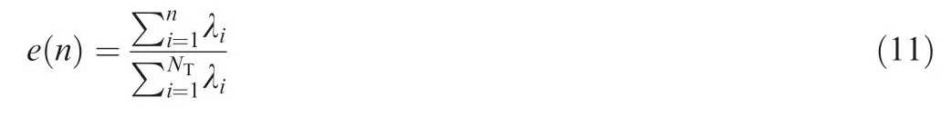
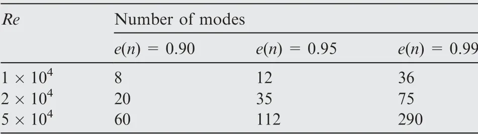
Table 1 Number of modes required as a function of Reynolds number and energy resolution.
describing the fraction of the kinetic energy captured by the firstnterm of Eq. (1). The increasing complexity of the flow is directly reflected to the fact that the number of modes required to reconstruct the same amount of kinetic energy increases non linearly. Here, we consider three families of models for every test case, resolving 0.90, 0.95 and 0.99 of the kinetic energy,respectively.The number of modes required to reach the requested energy resolution is shown in Table 1.
Once the coefficientsCi,LijandQijkin Eq.(3)are generated by Galerkin projection, the resulting system of ODEs can be integrated in time given one initial condition. In this work,an explicit time integration scheme with a time step of Δt=10-3time units has been used. All the systems have been integrated for a time span equal tot=100 time units,starting from an initial condition obtained from the DNS choosing a snapshot in the region of statistical convergence of the solution.Fig. 3 shows the temporal evolution of the turbulent kinetic energy as defined in Eq.(2)for three different ROMs resolving different amounts of kinetic energy and the baseline DNS. As expected,it is observed that the models reconstructing a lower amount of kinetic energy tends to overshoot the reference value of the turbulent fluctuations. This is a well know issue of reduced order modelling already discussed in Refs.14,20for POD-based models and is a direct consequence of the impossibility of dissipating the kinetic energy produced at the large scales in the small scales eliminated in the truncation process. As a result, the solution is not able to satisfy the energy balance of the original flow,presenting a higher energy in the first few modes associated with larger flow scales. More specifically, Fig. 3 shows that only thee(n)=0.99 model contains a sufficient number of modes to provide predictions comparable with the DNS.These results highlight that,in order to obtain reliable reduced order models,a large number of modes needs to be included,generating complex and computationally expensive models. The idea of sparsification consists in pruning the least important coefficients of the tensorQijkwithout truncate any mode from the original system. The desired outcome is to obtain accurate but computationally efficient models constructed by a large amount of modes(spatial scales)but containing only the relevant interactions.
3.2. Sparse regression
The sparse regression methodology was applied to the reduced order models withe(n)=0.90, 0.95 and 0.99, for the three Reynolds numbers. Since the relationship between number of modes and energy resolution is not linear and the size of the database matrix, Θ(A), increases quadratically withn, the number of possible interactionsqcan quickly become larger than the number of available snapshots,NT. This is a wellknown problem in statistical learning and requires crossvalidation methods to avoid data overfitting.24This work employs theK-fold validation procedure available in the sklearn library.38The database is divided intoK=10 folds.The model is initially trained on a subset of the entire database, obtained by removing thekth fold. Subsequently, the model is tested on thekth fold which was excluded for the model generation. The procedure is repeatedKtimes. To quantify the quality of the model predictions, the mean and standard deviation of the cross-validated reconstruction error,Eq. (8), are calculated over the folds.
The sparsification procedure consists in solving Eq. (7) for increasing values of the regularisation weight γ. Then the corresponding value of the density ρ and reconstruction error ε as defined in Eq.(9),Eq.(8)is computed and displayed on the ρ-ε plane.Fig.4 summarises the results of the sparsification procedure applied to the nine models considered.In each panel,the value of the mean cross-validated error ε against the density ρ is displayed for the three Reynolds numbers. The value of the resolved kinetic energy Eq. (11) increases from Fig. 4(a) to (c)showing the results fore(n)=0.90, 0.95 and 0.99, respectively.When low weights are used(right part of the panels in Fig.4),dense systems with low prediction error are obtained. The opposite is true for large weights, identifying points in the left part of the graphs. As postulated, since a set of coefficients in the tensorQijkis predominant,the curves present an initial plateau for high densities where it is possible to remove coefficients from the Eq. (3) without significantly affecting the reconstruction error ε.
Generally, the sparsification curves in Fig. 4 shown two emerging trends. First, the value of the reconstruction error ε in the plateau decreases monotonically as the energy resolution increases, since more modes participates in capturing the dynamics of the fluctuations.Secondly,and more importantly,the optimal density ρoptdecreases when the Reynolds number is increased. This can be observed qualitatively in Fig. 4 and more quantitatively later on in Fig. 5(a) showing the trends of ρoptagainst the value of the Reynolds number.These results show that more complex models can be more efficiently sparsified. There are two further considerations. For the model withe(n)=0.90 atRe=1×10⁴, no evident plateau exists in the ρ-ε curve,indicating that the reconstruction error increases as soon as coefficients are removed from the system.This phenomenon was also observed in Ref.31,and alerts that a successful sparsification may depend on the basis used in the model generation as well as the mathematical structure of the model.The second consideration relates to Fig.4(c).The curve for the model withe(n)=0.99 reveals a sharp elbow point, with an optimal density ρopt~0.1.After a short plateau,the reconstruction error increases, worsening predictions for denser models.This behaviour is due to the small amount of data confronted with the complexity of the system, and shows the importance of using cross-validation for systems of high complexity. It is important to underline that this effect is present only for the case at higher Reynolds number and energy resolution.Increasing the size of the dataset for the other models does not change significatively the shape of the curves.
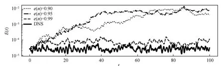
Fig. 3 Time evolution of turbulent kinetic energy at Re=2×10⁴ for reduced order models with different energy resolution and from DNS reference data.

Fig. 4 Mean of cross-validated reconstruction error against density of system.
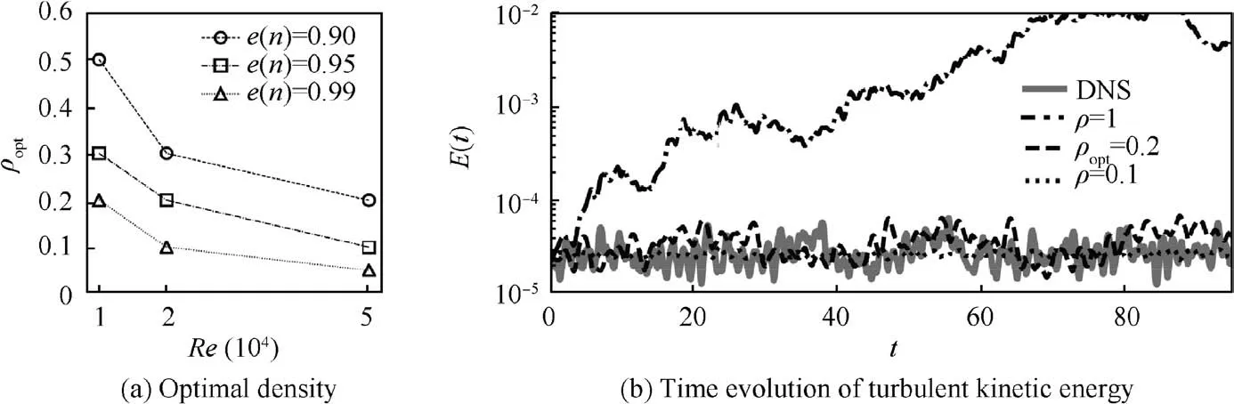
Fig. 5 Optimal density for all models considered in this study and time evolution of turbulent kinetic energy for three sparse models highlighted by circles in Fig. 4(b) compared to reference DNS.
To understand the effect of the sparsification on the temporal characteristics of the models,we analyse the temporal evolution of Eq. (2) for three different models chosen along the curves corresponding toe(n)=0.95 andRe=2×10⁴, shown in Fig. 5(b). The thee models corresponds to the three circles in Fig. 4(b) corresponding to the full system, a system located near the elbow point and one located in an area of very low density and with a higher error.Fig.5(b)shows that the behaviour of the dense system is qualitatively similar to that obtained by projection shown in Fig.3,leading to an overestimation of the kinetic energy of the flow.This result is expected since for ρ=1 the Eq. (7) is reduced to a pure least squares regression. More interestingly, decreasing the density of the model moving towards the sweet spot in the sparsification curves, the models’ predictions move closer to the DNS reference. Both sparse models seem to predict quite accurately the average kinetic energy level. However, a visual examination of the reconstructed vorticity field shows that for ρ=0.1 the main features of the flow are not reconstructed faithfully.Hereafter, we will only consider the optimally sparse model located in the proximity of the elbow point.Lastly,we observe that the value of ρoptdecreases as the Reynolds number increases. This is quantitatively shown in Fig. 5 (a) reporting the value of ρoptas a function of the Reynolds number. This effect is due to the broader range of scales in a model for increasing Reynolds number, and the weaker interactions among modes that are far in the spectrum.A qualitatively similar behaviour is observed increasing the energy resolution of the system. More importantly, this general trend shows that the effectiveness of the sparsification increases as the complexity of the model increases.
Fig. 6 shows time histories of the turbulent kinetic energy and the corresponding power spectral densities obtained by temporal simulation of models ate(n)=0.95 for the three different Reynolds numbers considered.DNS data is used as reference for two reduced order models: an optimally sparse model(black dashed curves),and a dense reduced order model(black curves). It is found that dense models overestimate the turbulent kinetic energy compared to DNS by several orders of magnitude. This is not unexpected because the model, not resolving the full range of scales of the flow,does not correctly model the energy dissipation occurring at the small scales. A confirmation of this observation can be seen in Fig.6(b),where the dense ROMs over-predict the energy content at all scales and for all Reynolds numbers. On the other hand,we observe that for the sparse models the level of the predicted kinetic energy is, on average, in agreement with the reference value.
To better visualise how the sparsification affects the predicted average kinetic energy,the ratiokrbetween the average reference kinetic energy and that predicted by the model is considered. The average has been computed fromt≥40, corresponding to the time needed by the solution to reach statistical convergence as can be observed in Fig. 6. Results are reported in Fig.7.Each panel displays data for six models,three dense models obtained by projection (empty triangles),and the corresponding sparse models with ρ=ρopt(full black circles). With optimal density we intend the sweet spot in the sparsification curves as shown in Fig. 4 (b). The Reynolds number increases moving from Figs. 7(a) to (c). A common trend for the three different flow conditions is observed. The models with a low energy resolution overestimate the fluctuating kinetic energy by two orders of magnitude. As the energy resolution of the model increases the value ofkrtends to values close to 1.This is an expected result since the number of spatial structures included in the model increases allowing the model to better describe the energy dissipation scales. Interestingly,for all sparsified models, the ratiokris close to 1. This means that on average the sparse system predict the right average amount of kinetic energy. In addition, we observe that the ratiokris almost constant as the energy resolution increases.This means that regardless the energy resolution chosen the LASSO optimisation problem (Eq. (7)) is able to provide correct predictions on the kinetic energy of the system. This is a direct consequence to the fact that the target of the acceleration is the modal accelerations ˙ai(t) computed from DNS simulation.
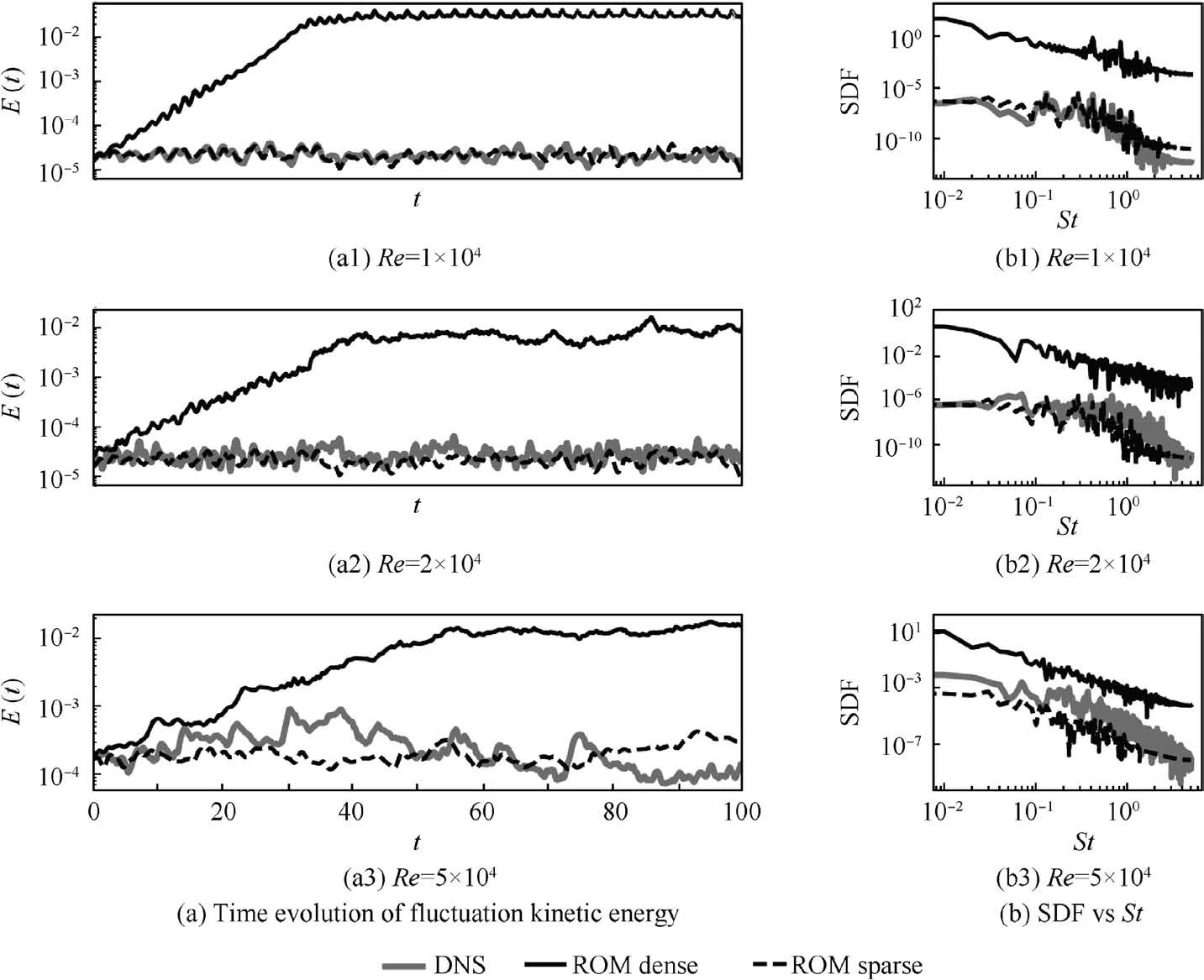
Fig.6 Time evolution of fluctuation kinetic energy E(t)and Spectral Density Function(SDF)of E(t)reported against nondimensional frequency St.

Fig. 7 Ratio kr for models with different energy resolutions e(n).
3.3. Reconstructed flow field
Once a solution of Eq. (7) is obtained, rearranging the coefficients vector βiinto a new set of matricessparse representation of Eq. (3) is obtained. The new dynamical system can be integrated to obtain the evolution of a new set ofai(t)that are used to reconstruct the flow field according to Eq. (1) since the spatial modes remain unchanged. Fig. 8 shows the reconstructed vorticity field ω for the optimally sparse models withe(n)=0.95.Every column contains results for a value of Reynolds number increasing from left to right.The top row shows the result of the time integration of the dense system while the bottom row shows the ones of the corresponding sparse model. From a visual analysis, we observe that the overshoot of kinetic energy observed in the dense models in Fig. 6 corresponds to non-physical large amplitude oscillations in the shear layer, as shown in Figs. 8(a) and (b), similarly for the model at highest Reynolds number the vortex in the lower right corner is amplified as well as shown in Fig. 8(c). This behaviour is due to an overestimation of the amplitude corresponding to the large and most energetic modes leading to an exaggeration of the low indexes modes as shown in Figs.2(b)-(d).More specifically,the sparse models reconstruct quite accurately the topology of the original flow field reproducing the shear layer and the vortex detachment for the lowest Reynolds numbers considered in Figs. 8(d) and (e). Similarly, for the highest value of the Reynolds number(Fig.8(f)),the sparse model is able to describe the formation and the shedding of the vortex produced in the bottom right corner of the cavity and subsequently shed and advected along the shear layer by the mean flow.

Fig. 8 Instantaneous snapshots of vorticity field ω.

Fig. 9 Profiles of Reynolds stress from simulation and from time integration of sparse and dense ROMs along line x=0.5.
A more in depth analysis on the dynamics of the velocity fluctuations can be done analysing the value of the time average of the Reynolds stressThis term is particular relevant for our analysis since the sparsification is performed on the set of Eq. (3) describing only the fluctuating part of the velocity field, while the mean field is left unchanged.
Fig.9 shows the profile of the Reynolds stress,along a vertical line located atx=0.5 for increasing values of the Reynolds numbers,from Figs.9(a)to(c).The grey continuous line is the reference from DNS while the optimally sparse model is represented as black dashed line.Results of the dense ROMs are reported as black dotted line in the background as reference. Since they are orders of magnitude larger than the ones observed in the DNS we chose a range of values on the horizontal axis in order to better visualise the results of the DNS and the sparse ROM.
For the two lower Reynolds numbers, Figs. 9(a) and (b),oscillations in the stresscan be observed, becoming more intense as the Reynolds number increases.In addition,outside the shear layer the stressdrops to zero except near the cavity lid. This result is expected since from a visual examination of Figs.1 and 8 we observe that outside the shear layer the flow is mainly stationary and presents quasi-periodic fluctuations.A different behaviour is shown in Fig. 8(c) for the highest Reynolds number.As already observed in Figs.1 and 8,in this case the shedding of the bottom-right vortex generates a much more complex flow field, with oscillations extended also near the central area of the cavity. For this flow configuration we observe that although the general distribution is reproduced the values are locally more different with respect to the other two test cases.
4. Conclusions
In this work a systematic data-driven methodology to perform sparsification and calibration of Galerkin based reduced order models of turbulent flows was utilised.The cornerstone of this approach consists in transforming the sparsification of a ROM into a convex optimisation problem independent from a priori knowledge on the flow physics.This methodology was applied to chaotic solutions of lid-driven square cavity flow. A family of POD-based Galerkin models with increasing complexity and spanning a range of Reynolds numbers and different energy resolution was created.Results show that pruning interactions from the original system does not affect the reconstruction error. The ρ-ε plane is used to identify the trade off between reconstruction error ε and system density ρ. It has been observed that when the Reynolds number or the energy resolution is increased, the optimal sparsity ρoptdecreases monotonically, showing that the sparsification becomes more efficient. Arguably, this behaviour is due to the widening of the range of dynamically active structures, generating a more pronounced decoupling between modes at different spatiotemporal scales.
A second important aspect is how the sparsification affects the temporal stability of the models.Interestingly,sparse models generally outperform the dense ones when it comes to the prediction of the average turbulent kinetic energy and its power spectrum.This improvement is due to the training phase of the sparsification algorithm,where the model is trained with respect to the DNS simulations.This allows the coefficients of the system to be calibrated to better describe the flow dynamics. This correction is more beneficial for models resolving a small amount of kinetic energy.This result was expected since for small ROMs energy dissipating scales are not resolved,generating an over-prediction of turbulent kinetic energy.
Lastly, the reconstructed flow field for the different Reynolds numbers was analysed. As expected, the overprediction of turbulent kinetic energy is reflected on the flow field as non-physical oscillations associated with the largest and low index modal structures.The sparsification is beneficial and allows reconstructing the flow structures observed in the DNS simulation. This is also confirmed by the distribution of Reynolds stresses in the shear layer;for the lowest Reynolds numbers these are in good agreement with the baseline DNS simulations. Differently, for the case at higher Reynolds number, the sparse model reproduces the magnitude of the Reynolds stresses while the spatial distribution is recovered only qualitatively. A visual examination of the flow fields shows that the key flow features,such as the formation and shedding of corner vortices, are recovered.
Looking further into the future,the proposed methodology serves as a key enabler for autonomous air and sea operations.The physics-informed model may be integrated into a cyberphysical model, for on-board and real-time applications. In this context, the cyber-physical model uses information derived from a network of sensors embedded on the system,at certain spatial locations. The measured information drives the reduced order model which reconstructs the flow state around the system,and feeds the state reconstruction to a mission manager.The mission manager,i.e.the‘‘brain”of the system,commands appropriate actions currently to match desired performance targets in the future using advanced navigation and guidance control laws, i.e. model reference adaptive control. This type of application is feasible in the near future by integrating commercial off-the-shelves hardware components into a flying testbed.
Declaration of Competing Interest
The authors declare that they have no known competing financial interests or personal relationships that could have appeared to influence the work reported in this paper.
杂志排行

CHINESE JOURNAL OF AERONAUTICS的其它文章
- Tangling and instability effect analysis of initial in-plane/out-of-plane angles on electrodynamic tether deployment under gravity gradient
- Aerodynamic periodicity of transient aerodynamic forces of flexible plunging airfoils
- Effects of swirl brake axial arrangement on the leakage performance and rotor stability of labyrinth seals
- Experimental and computational investigation of hybrid formation flight for aerodynamic gain at transonic speed
- Tomography-like flow visualization of a hypersonic inward-turning inlet
- Hypersonic reentry trajectory planning by using hybrid fractional-order particle swarm optimization and gravitational search algorithm