A swept fin-induced flow field with different height mounting gaps
2021-03-16FengZHANGShiheYIXiwangXUHaiboNIUXiaogeLU
Feng ZHANG, Shihe YI, Xiwang XU, Haibo NIU, Xiaoge LU
College of Aerospace Science and Engineering, National University of Defense Technology, Changsha 410073, China
KEYWORDS Fin;Flow visualization;Heat flux;Hypersonic;Shock/boundary layer interaction;Temperature sensitive paint
Abstract In order to apply the air fin successfully and ensure the maneuverability of hypersonic vehicle, a key problem to be studied urgently is the heat flux brought by the fin mounting gap.The appearance of mounting gap and fin shaft can induce many complex flow structures which need more attentions to be investigated.Under Ma 6,Nano-tracer-based Planar Laser Scattering(NPLS)and Temperature Sensitive Paints(TSP)were applied to visualize and measure transient flow structures and heat flux distribution of a swept fin-induced flow field with different height mounting gaps. Complementarily, Reynolds-averaged N-S equations were solved with k-ω SST turbulent model. The heat flux distribution results of numerical simulation and TSP observed the change of high heat flux region with different mounting gap,both in position and magnitude.The streamlines based on Computational Fluid Dynamics (CFD) and flow visualization results obtained by NPLS revealed the cause of high heat flux region. The high heat flux region in this flow field is mainly related to the reattachment of vortex and flow stagnation. The increase of gap height can lead to stronger gap overflow and shaft-induced horseshoe vortex,which are source of the high heat flux around the fin. The case with the highest mounting gap (4 mm) en-counters the most severe aerodynamic heating, both on the surface of fin and plate. Thus, under the premise of ensuring the flexibility of the fin, the gap should be set as small as possible.
1. Introduction
Hypersonic vehicles have become a major research field in aeronautics worldwide owing to their superior maneuverability,high level of survivability,and excellent global strike capability.1For controlling attitude and ensuring maneuverability,it is usually necessary to install various types of air fins on the surface of aircraft.2However, under hypersonic, there often exist many complex flow phenomena between the fins, wings and fuselage, such as shock/boundary layer interactions,shock/shock interference, boundary layer separation and reattachment, etc., which often lead to severe aerodynamic heating.3In addition, in order to ensure the flexible rotation of air fins and to accommodate the thermal expansion caused by the temperature rise of structures, it is necessary to reserve a certain height gap between the fin and the fuselage.Compared with mounting without gap, the one with gap is more complicated in the flow structures and aerodynamic heating.4Therefore,it is of great significance to study the influence of mounting gap on the flow field induced by fin.
The flow field induced by fin has been studied extensively in the past decades,5including the flow structures and heat transfer measurements. The studies on topological flow structures were mainly based on the numerical simulations,6-10as well as the inference from surface pressure measurements,11-14flow visualization results such as oil flow,15-17schlieren18and planar laser-induced fluorescence,19,20etc., and the separationshock, separation line and reattachment line around the fin are observed. In 1990, Stollery21summarized the topological structures of shock wave boundary layer interference flow field induced by blunt fin, and obtained the classical result, which consists of cross shock, separation shock, ‘‘λ” shock, horseshoe vortex and secondary vortex, etc. For measurements of heat flux caused by fin interference, the studies were more widely.16,22-27Lee22conducted an experimental research on the heat flux in three dimensional shock wave/boundarylayer interaction; he concluded that when an oblique shock wave impinges on a solid surface and interacts with the boundary-layer on that surface, a large separation bubble of reverse flow can form, generating a complicated three dimensional flow structure. The peak pressure, peak skin friction and peak heat transfer occur near the region of reattachment of this separated flow. Schuricht and Roberts23measured the interference heating effects generated by fin-type protuberances on hypersonic vehicles atMa6.7 with a model comprising a flat plate with a single, blunt fin using liquid crystal thermography. The results revealed a highly complex interaction region which extends 7 diameters upstream of the fin and with heating enhancements up to (and, in some cases,probably exceeding) 7 times the undisturbed value.
So far, there are only a few studies on the fin-induced flow field with mounting gap. In terms of experiments, Winkelman28studied the control fin with mounting gap on the missile,measured the influence of different gap sizes on the pressure and heat flux distribution of the flow, and found that large pressure peaks appeared near the high heat flux area, and the heat flux on the plate was 6 times of the non-interference value. Wieting et al.29carried out experiments on the flow and thermal environment of the gap in the forward wing span of elevator and the gap along the chord; they found that the thermal environment of the gap depended on the reflux and pressure difference. Li et al.30studied the aero-heating of the rudder shaft in shock wind tunnel,and found that the increase of the heat flux of the rudder shaft is larger under laminar flow conditions than that under turbulent flow conditions.In terms of simulation, Tan et al.31carried out numerical simulation of thermal environment for the hypersonic plate/fin model, and the influence of fin deflection angle, mounting gap height and the state of incoming boundary layer on the thermal environment of the fin shaft in the gap and the interference zone was analyzed. Huang et al.2studied the flow filed of a swept fin with mounting gap,using the finite volume method to solve the compressible Navier-Stokes equations, and found that the gap in blunt fin flow field make the flow structures more complex. The horseshoe vortex structure will appear in fin gap upstream, the shaft with the company of local high heat flux regions near the fin side.
On the whole, most studies on the flow field of hypersonic fins were focused on the fin without mounting gap.Studies on the influence of mounting gap on flow field of hypersonic fins are relatively scarce, especially the changes in the flow structures and aerodynamic heating caused by mounting gap. In this paper, under hypersonic condition, flow field structures induced by the fin with different mounting gaps are obtained based on Nano-tracer-based Planar Laser Scattering (NPLS)flow visualization technology with high spatial and temporal resolution. At the same time, the heat flux distribution of the interference area is measured by Temperature Sensitive Paints(TSP). The test results are compared with Computational Fluid Dynamics (CFD) results and the influence of mounting gap on flow structures and heat flux distribution of the swept fin induced flow field are depicted.
2. Model and flow conditions
2.1. Model
As is shown in Fig. 1, a blunt leading edge swept fin is mounted on a 400 mm long and 255 mm wide pointed leading edge plate through the fin shaft. The leading edge of fin is 125 mm away from the plate leading edge. The fin has a total length of 204 mm,a height of 83 mm,a leading edge radius of 3 mm and a sweep angle of 56°.The root thickness of the rear segment of the fin is 20 mm, so there is an expansion angle from the leading edge to the root. The position of the shaft is 260 mm away from the plate leading edge, and its diameter is 16 mm. By adjusting the height of the shaft, the adjustment of the height of the fin gaphcan be realized. The interference flow field of this swept fin under three different gap heights was studied experimentally. The gap height was 0 mm (that is, no fin gap), 2 mm and 4 mm respectively.
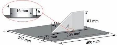
Fig. 1 Schematic of experimental model.
2.2. Wind tunnel and flow conditions
The experiments were carried out in theMa6 hypersonic low noise wind tunnel located at National University of Defense Technology. The wind tunnel is operated by blowing and suction. Its components include high-pressure air source, heater,setting chamber, hypersonic nozzle, test section and vacuum tank.Dry,clean air source and the nozzle which was designed based on a B-spline curve and made by special process ensure that the turbulence level of incoming free stream is lower than 0.3%. The length of test section is 700 mm, and the crosssection size is 260 mm×260 mm. Optical glass is installed in the side window of the test section, which facilitates the flow visualization and temperature sensitive paints tests. The wind tunnel is shown in Fig. 2. Due to the limitation of shooting angle,only the setting chamber,hypersonic nozzle and test section are included in the picture. The flow conditions of the experiment are shown in Table 1.
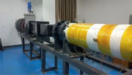
Fig. 2 Ma 6 hypersonic wind tunnel.
3. Experimental technique
Flow visualization experiments and heat flux measurement experiments were carried out on the carbon steel model and the bakelite model respectively. The structures of transient flow field were obtained by NPLS. And the heat flux distribution is measured by TSP.
3.1. NPLS
Since developed by Zhao et al.32in 2008, NPLS has been widely applied to studies on supersonic mixing layer,boundary layer transition, shock wave/boundary layer interference and supersonic cooling film, etc.32-35The components of NPLS system are shown in Fig. 3,including computer, synchronizer,CCD camera, pulsed laser and nanoparticle generator. The system uses double-cavity Nd:YAG laser to generate pulse laser, whose single pulse energy is 500 mJ with a 6 ns pulse width. After passing through the lens group, the laser beam is shaped into a sheet light with a thickness of 0.5 mm and illuminate the area of the flow field to be measured. A doubleexposure CCD is used to collect the scattering signals of particles, with a resolution of 2048 pixels×2048 pixels and a minimum interval of 200 ns. The precision of synchronization controller is up to 250 ps. According to the instructions set by computer, the trigger signal is sent to the laser and CCD to ensure that the light time of the laser is corresponding to the two exposures of the CCD, so that the scattering signals of particles under the two light beams are recorded in two images respectively. The nanoparticle generator distributes TiO2tracer particles with nominal diameter of 5 nm evenly mixing with the incoming flow. The computer is responsible for storing and analyzing the images captured by CCD and setting the synchronization parameters. During the experiment,the nanoparticles are injected by high-pressure gas and mixed with the incoming flow.Under the control of synchronizer,the double-cavity Nd:YAG laser outputs a pair of laser beams.The laser beam is converted into laser sheet through cylindrical lens, and when the beam illuminates the flow field, Rayleigh scattering will occur from the nanoparticles, thus producing the flow visualization image. The CCD camera is exposed according to the set time series, and the computer receives and stores the experimental images.

Fig. 3 NPLS system composition.
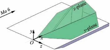
Fig. 4 Cartesian coordinate system.

Table 1 Flow conditions.
For a more intuitive description, a Cartesian coordinate system (as shown in Fig. 4) is established. The origin of the coordinate system is the intersection point of the fin central plane and the plate leading edge. Thex-axis follows the flow direction, they-axis is perpendicular to the plate, and thezaxis is determined by the right-hand rule.The flow field is visualized from thez-plane and they-plane which are commonly referred to as streamwise direction and spanwise direction.
In order to obtain the velocity information of flow structures based on time-correlation NPLS visualization images, a cross-correlation algorithm used in the field of image recognition was applied to NPLS images for the first time and obtained good results. This cross-correlation algorithm is called ‘‘Zero mean Normalized Cross-Correlation” (ZNCC),which matches the reference image and the target image based on gray scale. Its definition is as36
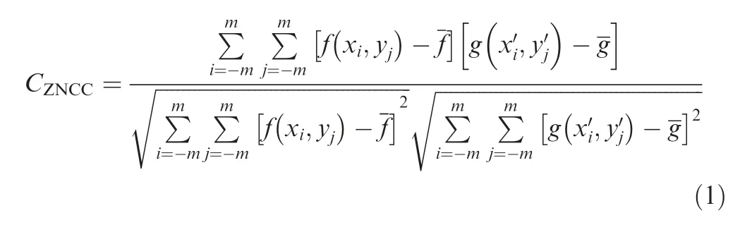
whereCZNCCis the correlation coefficient, the representation of the degree of correlation, whose maximum is at most 1;fandgrepresent the gray scale of the reference image and the target image at certain position respectively; (xi,yj) andare the pixel coordinates of the given points in the reference image and target image;mis 1/2 of the template size in the reference image and the superscript‘-’represents the mean of the template and the target region.
For example,a pair of time-correlation images of the turbulent boundary layer were obtained underMa6, as Fig. 5 shows. Its cross-frame time is 5 μs with the spatial resolution of 119.45 μm/pixel.Take a boxfintimage whose central point is 25.44 mm away from the wall as a template. The ZNCC method can find the target boxgin thet+5 μs image based on the maximum ofCZNCC, as Fig. 6 shows.
According to Fig. 6, the boxfhas moved 31 pixels inxdirection and 0 pixel inydirection within 5 μs,then the velocity offcan be calculated considering the spatial resolution. The velocity offis 740.59 m/s, which is about 0.881U∞.
3.2. TSP
In the long-duration wind tunnels, the temperature sensitive paints has been used for a long time.37TSP technique is based on the thermal quenching of luminescence of organic dye.When excited by LED light source, fluorescent molecules will emit long wave light, and the light intensity will decrease with the increase of temperature. Temperature and heat flux are measured according to this characteristic. The TSP developed by Changchun Applied Chemistry Institute was used. The paints were made by mixing adhesives with luminescent molecules and then dissolving them in a suitable solvent. To avoid the influence of oxygen quenching on the accuracy of temperature measurement, the adhesive must have oxygenimpermeability. Under this consideration, PolyVinyl Butanal resin (PVB) was selected as adhesive and the solvent was 99.9% anhydrous ethanol.

Fig.5 Time-correlation images of the turbulent boundary layer.

Fig. 6 CZNCC distribution versus dx and dy.
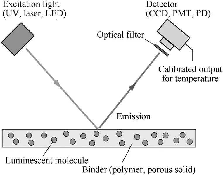
Fig. 7 Composition of TSP system.
A typical temperature sensitive paints system consists of the TSP coating, excitation light source, filter, detection and data acquisition system,as Fig.7 shows.The excitation light source used here is UV-LED with a single wavelength of 365 nm. At the same time,according to the luminescence characteristics of fluorescent molecule, a filter with the specification of 460 nm long wave pass was selected. For the detector, a CCD, a PhotoMultiplier Tube(PMT)or a Photo Detector(PD)is usually used.In this paper,a 12-bit CCD camera with a pixel resolution of 2048 pixels×2048 pixels was chosen as the detector,which can capture the light intensity of the TSP coating at 16 frames per second during the experiment.
Before the experiment, the surface of the model was uniformly sprayed with temperature sensitive paints with an airbrush, and then the model was placed in an incubator for several hours to dry. During the experiment, under the excitation light,the temperature sensitive paint coating emits fluorescence, whose intensity are concerned with the temperature around the fluorescent molecules. At the same time, its wavelength is usually longer than the excitation light,so it is convenient to detect and record the signal of emission light without the inference of excitation light using a suitable optical filter.Finally, after post process of the signal, the temperature and heat flux distribution of the model surface can be attained.
The static calibration of temperature sensitive paints coating was carried out in an incubator.A plate sprayed with temperature sensitive paints coating was put into the incubator,and the thermocouple was used to measure the accurate temperature.38The temperature of the TSP coating on the plate was adjusted by adjusting the temperature of the incubator.The temperature of the coating and the corresponding emitted light intensity under different temperatures were measured,and the relationship between the temperature ratio and the light intensity ratio can be gained through data postprocessing. 20°C was chosen as the reference temperature,and the calibration temperature range is 10-80°C with a calibration interval of 5°C. The calibration curve is shown in Fig. 8, whereIandTare the light intensity and temperature of TSP coating under experiment conditions;IrefandTrefare the reference light intensity and temperature of TSP coating under the reference temperature.
Within a certain temperature range,there is basically a linear relationship between the temperature change and the light intensity. As the temperature rises, the light intensity of TSP coating decreases linearly. By combining the calibration curve with the noise level of TSP,the temperature resolution of TSP was on the order of 0.5°C and the calibration curve equation is:39

After the temperature distribution is obtained from the TSP intensity,the heat flux distribution on the model surface can be calculated by the Cook-Felderman formula.40The discrete form of it is:

whereqw(t)represents the heat flux at timet;k,ρ andcrepresent the heat conductivity,density and specific heat capacity of the model material, respectively; ∇Twtiis the temperature change of the TSP coating at timeti.
The heat flux results measured by TSP are dimensionless in the form of Stanton number (St), which is defined as:

whereqwis the heat flux calculated according to the results of TSP; ρ∞,u∞andcpare the density, velocity and specific heat capacity at constant pressure of free stream respectively;Twis the wall temperature.Flow density ρ∞and velocityu∞can be calculated by isentropic relationship.
4. Numerical simulation
The Fluent V18.0 steady-state implicit solver was used in numerical simulation to solve the Reynolds Averaged N-S(RANS)equation.Among them,the gradient term of the flow field adopts the node-based Green-Gaussian space dispersion method, and the flux term adopts the AUSM flux format invented by Liou et al.41with the second-order upwind. Thek-ω SST model is applied, which is considered suitable for the calculation of separation flow and heat flux.4,42
The model used in numerical simulation is consistent with the experiment, including the location of the model and the size of the experimental section. The inlet and outlet are both 260 mm×260 mm. Meanwhile, the distance from the inlet to the leading edge of the plate and the trailing edge of the plate to the outlet are 200 mm.
The boundary conditions of the numerical simulation are set as follows:the inlet is defined as the pressure inlet.To generate the incoming flow ofMa6, the total pressure is set to 0.6 MPa, and the static pressure is set to 380 Pa with the total temperature 400 K.The outlet is defined as pressure outlet and the static pressure is 380 Pa.The total temperature of outlet is 298.15 K, consisting with room temperature. The surface of fin, shaft, flat plate and wind tunnel wall are defined as nonslip isothermal wall, and the temperature is also 298.15 K.The boundary conditions are simply labeled in Fig. 9.
Using commercial software ANSYS ICEM to generate structural grids,approximately 9.7 million mesh cells were generated in the computational domain in order to obtain sufficient spatial resolution. For the grid encryption near the surface of the plate,fin body and fin shaft,1.05 times of expansion ratio was used to analyze the boundary layer. The height of the first layer grid was guaranteed toy+ less than 0.2 to ensure that it was sufficient to solve the temperature boundary layer.42
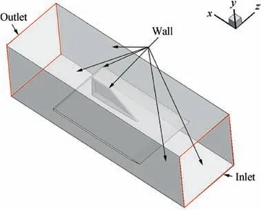
Fig. 9 Model and boundary conditions for simulation.
A grid convergence study was performed based on theh=0 mm case. Three grids of approximately 3.25, 5.62, and 9.70 million cells were used for the grid convergence investigation, using a grid refinement ratior=1.2 in all three grid directions. The convergence was assessed in terms of static pressure distribution alongx-axis on plate atz=20 mm,which is shown in Fig.10.The maximum relative errors among them all appear atx=0.323 m, and the relative errors were presented in Table 2. The relative error between the medium and the fine grid solution is below 0.48%,which is satisfactory.The numerical results are all based on the fine grid, and the convergence condition of iterative is that the mass residual and momentum residual are less than 10-6, and the energy residual is less than 10-7.

Fig. 10 Static pressure (P) distribution along x-axis on plate at z=20 mm.

Table 2 Grid convergence parameters for the three grids.
5. Results and analysis
5.1. Flow visualization results of incoming boundary layer and the fin symmetrical plane
Flow visualization of the incoming boundary layer under experimental conditions was carried out based on NPLS.The flow state and thickness of the plate boundary layer, at the leading edge position when the swept fin were mounted,were obtained. As shown in Fig. 11, atx=125 mm where the leading edge of the swept fin is located, the incoming boundary layer is a stable laminar flow with a thickness about 2.1 mm.
The flow field is studied under the mounting gap of 0 mm,2 mm and 4 mm, whose correspondingh/δ is 0, 0.95 and 1.90 respectively, where δ is boundary layer thickness. The corresponding flow visualization results of the fin symmetrical plane are shown in Fig. 12, from which we can see that, there is no significant difference of the leading edge shock and the bow detached shock among those conditions.The difference is that the existence of mounting gap makes part or all of the incoming boundary layer flow downstream through the mounting gap, and the boundary layer separation near the leading edge of the swept fin weakens or even disappears. Inh=4 mm case, for the gap height is higher than the incoming boundary layer thickness,all incoming boundary layer flows downstream through the gap, and no separation occurs near the leading edge.
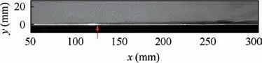
Fig. 11 Incoming boundary layer.

Fig. 12 Flow structures of fin symmetry plane.
5.2. Results for the flow field without mounting gap
5.2.1. CFD results of streamlines and Stanton number distribution for h=0 mm case
When the hypersonic flow is hindered by fin, a bow detached shock will form at the leading edge. As the bow shock penetrates into the boundary layer of the incoming flow,a‘λ’shock is formed. A separation zone usually appears in the structures of the‘λ’shock,whose high vorticity often leads to the formation of horseshoe vortex.21Fig. 13 shows the streamlines and Stanton number contours around the fin based on CFD.Hypersonic flow is hindered by fin,resulting in separation lineS1. The separation pointSis located at aboutx=123.5 mm in the symmetry plane,only 1.5 mm from the fin leading edge.The separation flow reattaches atRon leading edge, only 2.8 mm to fin root. The reattachment flow separates atS2(shown in Fig. 14) during passing the fin, and then reattaches on the plate, forming the reattachment lineR1. To facilitate quantitative comparison, the positions ofS1andR1were extracted: forx=200 mm,S1is atz=±35.9 mm,R1is atz=±8.5 mm; forx=280 mm,S1is atz=±54.0 mm,R1is atz=±18.8 mm.
FromStcontours, three high heat flux regions can be observed, namely,H1,H2andH3. Among them,H1which nears the leading edge and along the outside ofR1has the highest magnitude, about 1.88×10⁻³. Continue downstream,H2andH3are located on either side ofR1,whose magnitudes are 1.21×10⁻³and 9.3×10⁻⁴respectively.
Fig.14 shows the streamlines and Stanton number distribution on the lateral surface of fin. Forh=0 mm case, there is no obvious high heat flux region on the lateral surface of fin.The separation lineS2is the only characteristic on the lateral surface,which is caused by the retardation of the reattachment flow from the leading edge due to the vortex in the fin corner,as Fig. 15 shows.

Fig. 13 Streamlines and Stanton number distribution around the fin (h=0 mm, CFD).
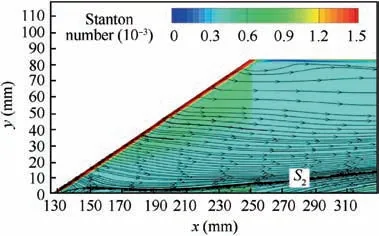
Fig. 14 Streamlines and Stanton number distribution on lateral surface of fin (h=0 mm, CFD).
Fig. 16 shows the NPLS images of the flow structures around the fin without mounting gap.The laser sheet of NPLS is 2 mm away from the plate and the time interval of upper and lower image is 5 μs. In Fig. 16, the continuous horseshoe vortex induced by the separation zone of the leading edge can be clearly observed.Horseshoe vortex is generated from the leading edge separation zone with a small scale in initial state, but with the development of flow field to the downstream,the size of vortex gradually increases.Based on the ZNCC method,the streamwise velocityuand spanwise velocitywof the horseshoe vortex ata1,b1andc1were obtained,with(u,w)=(192.7 m/s,48.2 m/s),(337.3 m/s,24.1 m/s),(457.7 m/s,-24.1 m/s)respectively.With the development of horseshoe vortex,the vortex is mixed with the mainstream gradually, and the streamwise velocity increases. At the same time, under the effect of the pressure gradient pointing to the fin, the spanwise velocity gradually decreases until near the fin tail.Due to the existence of the low pressure region near the fin tail, the direction ofwchanges, and the horseshoe vortex flows to the low pressure area near the tail. Atx=200 mm, the horseshoe vortex is betweenz=± (22-24) mm, that is, approximately locates in the midline of separation lineS1(z=±35.9 mm)and reattachment lineR1(z=±8.5 mm) in Fig. 13. Atx=280 mm,the horseshoe vortex is betweenz=± (19-40) mm. With the scale increasing of vortex,its central position deviates from the midline position of separation lineS1(z=±54.0 mm)and reattachment lineR1(z=±18.8 mm), and moves slightly to the reattachment line.

Fig. 15 Streamlines near the leading edge of fin (h=0 mm,CFD).

Fig. 16 Time-evolution of the flow structures around fin(h=0 mm, y=2 mm).
5.2.3. Stanton number distribution measured by TSP for h=0 mm case
Fig. 17 shows the Stanton number distribution on the surface of flat plate forh=0 mm case.At the outermost side of the fin is an arched heat flux regionA, whose amplitude is slightly higher than its surrounding area and slowly rises with the development of the flow to the downstream. On the fin side near the leading edge,there is a small high heat flow regionB,whose Stanton number distribution is shown in Fig. 18(a),with a peak heat flux of 1.82×10⁻³at (x,z)=(140.1 mm,5.5 mm). RegionBis located near the reattachment lineR1in Fig. 13 and is likely caused by the reattachment of the hot flow from fin leading edge. Within the range ofx=180-210 mm andz=± (7-12) mm, is another heat flux regionCwith a peak value of 1.80×10⁻³(seen in Fig. 18(b)). At the same time,as the flow brings the heat in regionCdownstream,a decreasing high heat flux regionDyields. Atx=200 mm,regionAis betweenz=± (21 - 27) mm, which is approximately located in the middle line of separation lineS1and reattachment lineR1. RegionCis betweenz=± (7-12) mm,corresponding to the reattached lineR1in Fig. 13.Atx=280 mm, regionAis betweenz=± (36-42) mm,which is also basically located in the middle line of separation lineS1and reattachment lineR1, while regionDis betweenz=± (18-28) mm, which is adjacent to reattachment lineR1and may be caused by the reattachment of horseshoe vortex to the reattachment line. Compared to theStdistribution shown in Fig. 13, there is some difference between experiment and simulation results, especially in the position of high heat flux region, which may remind us that the calculation of heat flux by numerical simulation still needs further improvement.
Meanwhile, the Stanton number distribution on the lateral surface of fin is shown in Fig.19.Similar to Fig.14,there is no obvious high heat flux region can be observed on the lateral surface of fin. Only a band of a little high heat flux near the fin foot can be observed, and its peak value is only about 8×10⁻⁴.
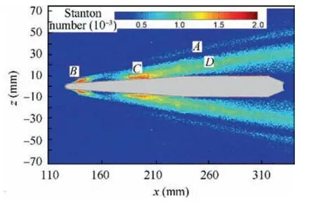
Fig.17 Stanton number distribution on flat plate surface around fin (h=0 mm, TSP).
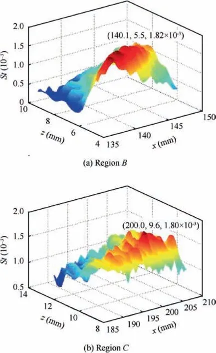
Fig. 18 Stanton number distribution in high heat flux region.
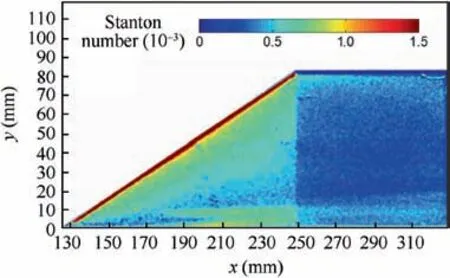
Fig.19 Stanton number distribution on the lateral surface of fin(h=0 mm, TSP).

Fig. 20 Streamlines and Stanton number distribution around the fin (h=2 mm, CFD).
5.3. Results for the flow field with 2 mm mounting gap
5.3.1. CFD results of streamlines and Stanton number distribution for h=2 mm case
Fig.20 shows the streamlines of the flow field induced by swept fin with 2 mm mounting gap. Underh=2 mm, part of the incoming boundary layer can flow downstream through the gap. Thus, the blockage to incoming boundary layer caused by the fin is weakened. The separation point in the symmetry plane is already inside the gap, which is at aboutx=129.2 mm, 4.2 mm downstream of the fin leading edge.The reattachment point is also inside the fin gap,approximately atx=131.7 mm, 6.7 mm downstream of the fin leading edge. The reason why separation point and reattachment point are inside the fin gap is the root of fin leading edge,which hinders the supersonic flow and produces a leading edge shock wave inside the gap. The shock wave acts on the plate boundary layer in the gap, and then, the boundary layer separates.The spanwise positions ofS1andR1atx=200 mm arez=±33.2 mm andz= ±10.8 mm respectively.
The gap flow continues to flow downstream, and then blocked by the shaft. Due to supersonic flow inside the gap,flow structures,similar to that around the cylinder,43,44is generated near the shaft. The gap flow separates at aboutx=235 mm, producing the separation lineS2. After that, the gap flow reattaches at aboutx=250 mm, which is only 2 mm away from the surface of the shaft, producing the reattachment lineR2. Under the influence of the separation flow induced by shaft, the upstream reattachment lineR1begins to diverge near the separation lineS2, and the lateral flow of the fin can no longer reattaches normally.The position ofS1also moves away from the fin due to the influence of the separation flow of the shaft. Atx=280 mm,S1is located atz=±54.8 mm,S2is located atz=±36.5 mm, andR2is located atz=±24.2 mm.
FromStcontours, four high heat flux regions can be observed.H1is near the leading edge and along the reattachment lineR1, whose peak value appears between the gap andR1and increases to about 1.99×10⁻³compared to Fig. 13.The increase ofStmay be caused by the combined effect of reattachment flow from leading edge and the overflow from mounting gap.In the middle of fin,lateral side of the mounting gap is the high flux regionH2with a magnitude of 1.34×10⁻³.H3is the region near the fin shaft, whose magnitude is 1.45×10⁻³. Meanwhile,H4is along the reattachment lineR2, with a peak value about 1.38×10⁻³.
Fig.21 shows the streamlines and Stanton number distribution on the lateral surface of fin. Underh=2 mm case, separation lineS3caused by the flow around the shaft can be easily recognized. Atx=230-250 mm, the heat flux caused by the separation flow around the shaft can be observed,with a peak value about 1.05×10⁻³.
5.3.2. Flow visualization results around the fin for h=2 mm case
Fig. 22 shows the flow structures around the fin with 2 mm gap. The laser sheet of NPLS is located at the central of gap,that is, 1 mm away from the plate. Due to the existence of gap, the boundary layer separation upstream of the fin weakens and the horseshoe vortex becomes less obvious. The growth rate of vortex is accelerated with the downstream development of the flow field and the influence of the down-stream fin shaft separation flow. The streamwise velocityuand spanwise velocitywof the horseshoe vortex ata2,b2andc2are (u,w)=(289.1 m/s, 48.2 m/s), (530.0 m/s, 144.5 m/s),(626.3 m/s, 48.2 m/s) respectively. Under the action of flow around shaft, the spanwise velocity of horseshoe vortex increases obviously than that of 0 mm.The gap flow is blocked by the downstream separation flow of shaft, and some gap overflow occurs at the fin side, resulting in a small amount of overflow vortices. Horseshoe vortex is generated from the separation zone inside the gap. The velocity of vortexd2is(770.8 m/s, 24.1 m/s), which can be an evidence of the appearance of gap overflow. Because the boundary layer is very thin near the fin,the overflow velocity is very high and it is easy to affect the wall.The velocity of the horseshoe vortexe2around shaft is (770.8 m/s, 120.4 m/s). Such a high spanwise velocity demonstrates that the shaft has a considerable effect on the flow in its vicinity. The influence of the shaft separation flow even exceeds that of the fin. Atx=200 mm, the spanwise position of the horseshoe vortex is betweenz=± (23 -28) mm. Upstream of the fin shaft, aboutx=180-230 mm,the gap flow is affected by the separation zone of the downstream fin shaft, resulting in a certain scale of overflow at the fin side. In the vicinity of the shaft, aboutx=230-240 mm, the flow in the gap separates, and the second horseshoe vortex is generated by the separation flow. According to rough estimation, the spanwise position of first horseshoe vortex is betweenz=± (34-46) mm, and its central position moved away from the fin significantly than the state without gap. The spanwise position of the second horseshoe vortex is betweenz=±(24-36)mm,and its central position is approximately at the median line betweenS2(z=±36.5 mm) andR2(z=±24.2 mm) in Fig. 20.
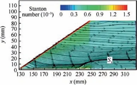
Fig. 21 Streamlines and Stanton number distribution on lateral surface of fin (h=2 mm, CFD).

Fig. 22 Time-evolution of the flow structures around fin(h=2 mm, y=1 mm).
5.3.3. Stanton number distribution measured by TSP for h=2 mm case
Fig.23 shows the Stanton number distribution on plate surface around the fin with 2 mm mounting gap.The range of regionBnear the leading edge has slightly extended thanh=0 mm case, and its peak value also slightly increases to about 1.93×10⁻³(shown in Fig. 24(a)). RegionCin the middle of fin side is affected by the overflow of gap and the separation zone of the downstream fin shaft.Its position moves upstream and the range extends, ranging fromx=167-230 mm andz= ± (4 - 26) mm, with the peak value rises to about 1.88×10⁻³(shown in Fig. 24(b)). At aboutx=230 mm, the shaft separation flow begins to dominate the heat flux distribution in the region around the shaft,and a high heat flux regionEis generated near the shaft, with a small range of aboutx=233-253 mm andz=± (10-14) mm, and a peak value of 1.90×10⁻³(shown in Fig. 24(c)). The shaft separation flow develops downstream, and generates the second horseshoe vortex, which causes heat flux regionD.Atx=200 mm, regionAis betweenz=± (23-27) mm,which moves slightly laterally compared to that without mounting gap. RegionCis betweenz=± (7-19) mm, which is also near the reattachment lineR1in Fig. 20. However, due to the gap overflow,the distribution of heat flux regionCis on both sides of the reattachment lineR1.Atx=280 mm,regionAis betweenz=±(40-45)mm,which also moves slightly laterally. RegionDis betweenz=± (18-32) mm, which is distributed on both sides of the reattachment lineR2,and its peak position basically coincides with that of the reattachment lineR2, about 1.2×10⁻³.
The Stanton number distribution on the lateral surface of fin is shown in Fig. 25. Atx=210-250 mm, the heat flux regionFcaused by the separation flow around the shaft can be observed,with a peak value about 1.25×10⁻³.The magnitude of heat flux regionC,EandFare higher than CFD results obviously, from which we can speculate that the influence of shaft is more significant in experiments than simulations.

Fig.23 Stanton number distribution on flat plate surface around fin (h=2 mm, TSP).
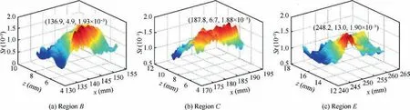
Fig. 24 Stanton number distribution in high heat flux region.

Fig.25 Stanton number distribution on the lateral surface of fin(h=2 mm, TSP).
5.4. Results for the flow field with 4 mm mounting gap
5.4.1. CFD results of streamlines and Stanton number distribution for h=4 mm case
Fig.26 shows the streamlines of the flow field induced by swept fin with 4 mm mounting gap. Under this condition, all the boundary layer of incoming flow can flow downstream through the gap. The separation point ofS1in the central plane moves downstream further inside the gap,approximately atx=133.6 mm,about 8.6 mm downstream from the leading edge. The reattachment point in the central plane also moves downstream to aboutx=135.8 mm, about 10.8 mm downstream from the leading edge. Atx=200 mm,S1is located atz=±32.9 mm,R1is located atz=±11.1 mm.
Since the flow velocity in the gap is higher than that under the condition of 2 mm gap, stronger separation is generated near the fin shaft. The separation position is aboutx=231 mm, and the separation lineS2is generated.After that, the gap flow is reattached at aboutx=251 mm,only 1 mm away from the surface of the shaft, resulting in the reattachment lineR2. Influenced by the separation flow of the fin shaft, the divergent position of the upstream reattachment lineR1moves further upstream, and the position of the separation lineS1is further away from the fin.Atx=280 mm,S1is located atz=±57.5 mm,S2is located atz=±48.0 mm,andR2is located atz=±23.2 mm.It can be seen that in the condition of 4 mm gap, the strong separation of the flow near the fin shaft makes the separation linesS1andS2far away from the fin, while the reattachment lineR2is closer to the fin.
From the Stanton number contours, we can see that the magnitude of regionH1andH2decrease obviously compared toh=2 mm case. However, the peak value ofH3andH4increase significantly to 2.04×10⁻³and 2.15×10⁻³. The higher gap leads to much stronger separation flow around shaft, which causes the severer aerodynamic heat.

Fig. 26 Streamlines and Stanton number distribution around the fin (h=4 mm, CFD).
Fig.27 shows the streamlines and Stanton number distribution on the lateral surface of fin. Underh=4 mm case, separation lineS3caused by the flow around the shaft moves further away from the shaft,indicating the stronger separation appears.Atx=230-260 mm,the heat flux caused by the separation flow around the shaft is much more obvious.With the extension of the area being influenced, its peak value reached terrible to 2.33×10⁻³, which is even higher than that ofH4in the plate.
5.4.2. Flow visualization results around the fin with for h=4 mm case
Fig.28 shows the spanwise flow structures around the fin with 4 mm gap.The laser sheet of NPLS is located at the central of the gap, that is, 2 mm away from the plate. As the gap size increases, all the incoming boundary layer flows downstream through the gap,and the strength of the first horseshoe vortex is further lower. The velocity of gap flow is higher thanh=2 mm case,and when it is blocked by the downstream separation flow around shaft, the scale of gap overflow at the fin side appears much larger, forming stronger overflow vortices.The velocity of gap overflow structuresa3anddare(626.3 m/s, 96.4 m/s), (699.3 m/s, 72.3 m/s). The loweruand the higherwprove that the gap flow is more affected by the separation flow of shaft thand2inh=2 mm case, and the gap overflow becomes stronger. The horseshoe vortex is outside the overflow vortex, and atx=200 mm, the spanwise position of the horseshoe vortex is atz=± (26-28) mm.Influenced by the overflow vortex, the spanwise position of the horseshoe vortex obviously moves away from the fin.Upstream of the shaft, at aboutx=230 mm, gap flow separates with a significantly larger separation strength. The scale of the second horseshoe vortex is very obvious. The velocity of the second horseshoe vortex ate3,b3andc3are (554.0 m/s,192.7 m/s), (530.0 m/s,144.5 m/s) and (457.7 m/s, 120.4 m/s).The streamwise velocity and spanwise velocity all decrease gradually with the development of vortex to the downstream.These velocity data all indicate that the strength of the separation vortex of shaft is much higher than that ofh=2 mm case.Atx=280 mm, the first horseshoe vortex has mixed with the second horseshoe vortex. Estimating roughly, the first horseshoe vortex spanwise position isz=±(42-52)mm,its central is further away from the fin.The spanwise position of the second horseshoe vortex is betweenz=± (26-46) mm, and its central position is approximately at the median line betweenS2(z=±48.0 mm) andR2(z=±23.2 mm).

Fig. 27 Streamlines and Stanton number distribution on lateral surface of fin (h=4 mm, CFD).

Fig. 28 Time-evolution of the spanwise flow structures around fin (h=4 mm, y=2 mm).
5.4.3. Stanton number distribution measured by TSP with for h=4 mm case
Fig. 29 shows the Stanton number distribution on the plate surface around the fin with 4 mm mounting gap. With the increase of gap height, the bow heat flux regionAis almost invisible. After the emergence of separation flow induced by the shaft, it can be recognized hardly. The increase of gap height makes the gap overflow more intense,and the reattachment heat flux regionBnear the leading edge has disappeared.The position of regionCcontinues to move upstream, and its range continues to expand, which is distributed with an expanding triangle in the range ofx=130-230 mm,however,its peak value is reduced to about 1.38×10⁻³(shown in Fig. 30(a)). Downstream ofx=225 mm, the separation flow of the shaft causes the heat flux near the shaft rise sharply.The high heat flux regionEnear the shaft and the regionDcaused by the horseshoe vortex generated by separation flow have been integrated, and the peak value has reached 2.11×10⁻³and 2.33×10⁻³respectively(shown in Fig.30(b)),a little higher than CFD results. Atx=280 mm, the position of regionAisz=±(48-52)mm,which is pushed by the separation flow induce by shaft, thus, regionAmoves to the lateral direction obviously. The spanwise range of regionDcaused by horseshoe vortex isz=± (16-40) mm.
The Stanton number distribution on the lateral surface of fin is shown in Fig. 31. The heat flux regionFcaused by the separation flow around the shaft is much more obvious. With the extension of the area, its peak value reached terrible to 2.43×10⁻³, also a little higher than CFD results in Fig. 27 and regionDin Fig. 29. Outside of regionF, there is another heat flux bandG,whose magnitude is 8.1×10⁻⁴,which is not very obvious.
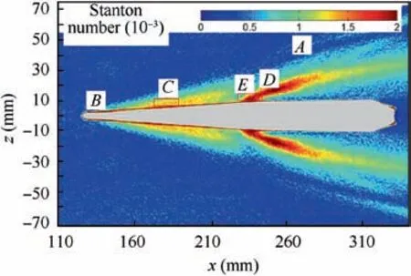
Fig.29 Stanton number distribution on flat plate surface around fin (h=4 mm, TSP).

Fig. 30 Stanton number distribution in high heat flux region.

Table 3 z-position statistics at x=200 mm.

Table 4 z-position statistics at x=280 mm.
5.5. Comparison and analysis
In order to conclude the positional relationship among separation line,reattachment line,vortex structure and high heat flux region,we made statistics of such information and got Tables 3 and 4, wherex=200 mm data was shown in Table 3,andx=280 mm data was shown in Table 4. The location data in the table unified on one side, only taking the positive direction of thezaxis.
As shown in Tables 3 and 4, the horseshoe vortex usually appears between the separation line and reattachment line,with its central line usually closer to the reattachment line.The position of high heat flux region is closely related to the location of vortex,and often closer to the side of reattachment line at the mean time.
Another reality which we need to recognize is that the high heat flux region where the most severe aerodynamic heating appears is often related to the stagnation of the flow. For example, inh=0 mm case, the peak value ofStis in regionB,which is caused by the reattachment of the hot flow passing through the leading edge, where the stagnation appears.
Based on previous analysis, the characteristic of the fininduced flow field with different height gaps can be summarized as follows:
(1)h=0 mm case
The incoming boundary layer separates from the leading edge, which develops into a continuous horseshoe vortex with increasing scale downstream.The horseshoe vortex causes two heat flux regions around the fin. The outermost heat flux region has a low strength and develops downstream in a bow shape,while the inner heat flux region has a higher magnitude and its position is around the edge of the horseshoe vortex and near the reattachment line.
The separation flow on the symmetry plane reattaches at the leading edge of the fin. Then, it forms the lateral flow around the fin and reattaches atR1, resulting heat flux regionBand regionCon the plate.The magnitude of regionBis the highest, with a peak value of 1.82×10⁻³.
Forh=0 mm case,there is no high heat flux appearing on the lateral surface of fin.
(2)h=2 mm case
Part of the incoming boundary layer flows downstream through the gap.Subjected to shock wave,the boundary layer separates inside the gap. A continuous horseshoe vortex with the increasing scale also appears. For the gap height is relatively small, the hot flow from leading edge and the gap overflow reattach atR1simultaneously, increasing the magnitude of regionBto 1.93×10⁻³.
The gap flow is blocked by shaft and form the shaft separation flow. Upstream the separation flow, gap overflow occurs.The gap overflow and the flow from the leading edge reattach atR1in the meantime,which increases the peak value of regionCto 1.88×10⁻³.The gap flow impinges on the shaft, causing heat flux regionE,with a peak value of 1.90×10⁻³.While the shaft separation flow towards downstream,horseshoe vortex 2 causes the heat flux regionD.
Forh=2 mm case,a relative high heat flux appears on fin lateral surface near the shaft,with a magnitude of 1.05×10⁻³.The heat flux level is not serious.
(3)h=4 mm case
All the incoming boundary layer flows downstream through the gap. Due to the increase of gap height and the higher strength of gap overflow, the airflow from the leading edge is difficult to reattach atR1, thus the heat flux regionBdisappears.The enhancement of the gap overflow caused a further expansion of heat flux regionC, but the heat flux caused by gap overflow is lower than that of the flow from the leading edge, and the peak ofStis reduced to 1.38×10⁻³.
The increase of gap height makes the shaft separation flow more intense.The separation lineS2moves further away from the fin, while the reattachment lineR2moves closer to the fin.The gap flow impinges on the fin shaft, causing heat flux regionEaround the shaft and regionDdownstream,whose peak value reach 2.11×10⁻³and 2.33×10⁻³respectively.
Forh=4 mm case, the high heat flux appears on fin lateral surface near the shaft is very severe, with a magnitude of 2.43×10⁻³, even exceeding the heat flux level on the plate.
6. Conclusions
In order to study the influence of the mounting gap on flow structures and heat flux, provide guidance for the design and thermal protection of hypersonic vehicles, the flow structures and heat flux distribution of a swept fin induced flow fields were visualized and measured with different height mounting gaps in aMa6 hypersonic wind tunnel. Through the contrastive analysis of the experimental results and the numerical simulation, the following conclusions can be concluded:
(1) Without mounting gap, the high heat flux region in swept fin induced flow field is mainly caused by reattachment of the flow from the fin leading edge, with a peak value of 1.82×10⁻³.The incoming boundary layer separates and causes the horseshoe vortex, but its heat flux intensity is low.
(2) With 2 mm gap, the flow field contains three high heat flux region with similar intensity, which are respectively caused by the reattachment flow from the fin leading edge,the combination of gap overflow with fin side flow reattachment, and the gap flow impingement on fin shaft, with a peak value about 1.90×10⁻³.
(3) With 4 mm gap, the impingement heat flux near the shaft and the heat flux caused by the accompanying horseshoe vortex increases sharply, whose peak value has reached 2.11×10⁻³and 2.33×10⁻³respectively.The high heat flux appears on fin lateral surface near the shaft is even severer, with a magnitude of 2.43×10⁻³.
(4) The heat flux distribution is closely related to the vortex.The reattachment of vortex to reattachment lines often leads to high heat flux.
In summary,under the premise of ensuring the flexibility of the fin, the mounting gap should be set as small as possible to avoid high heat flux,which reduces the cost of thermal protection and ensures the structural safety of the aircrafts.
Declaration of Competing Interest
The authors declare that they have no known competing financial interests or personal relationships that could have appeared to influence the work reported in this paper.
Acknowledgements
This work was supported by the National Key Technology Research and Development Program of China (No.2019YFA0405300), the National Project for Research and Development of Major Scientific Instruments of China (No.11527802) and the National Natural Science Foundation of China (No. 11832018).
杂志排行

CHINESE JOURNAL OF AERONAUTICS的其它文章
- Tangling and instability effect analysis of initial in-plane/out-of-plane angles on electrodynamic tether deployment under gravity gradient
- Aerodynamic periodicity of transient aerodynamic forces of flexible plunging airfoils
- Effects of swirl brake axial arrangement on the leakage performance and rotor stability of labyrinth seals
- Experimental and computational investigation of hybrid formation flight for aerodynamic gain at transonic speed
- Tomography-like flow visualization of a hypersonic inward-turning inlet
- Hypersonic reentry trajectory planning by using hybrid fractional-order particle swarm optimization and gravitational search algorithm