GRADIENT ESTIMATE FOR POSITIVE SOLUTIONS OF THE PME UNDER GEOMETRIC FLOW

ZHAO He-lei

(School of Mathematics and Statistics,Wuhan University,Wuhan 430072,China)

Abstract:In this paper,we derive a local gradient estimate of the Aronson-B´enilan type with Laplace operator and drifting Laplace operator for positive solutions of porous medium equations posed on Riemainnian manifolds with bounded symmetric tensor by using Li-Yau method.These results extend Zhu Xiao-bao’s and Deng Yi-hua’s results.

Keywords:gradient estimate;geometric flow;porous medium equations;Harnack inequality

1 Introduction

The porous medium equation(PME for short)

appears in the description of different natural phenomena,and its theory and properties depart strongly from the heat equation,ut= ∆u,it’s most famous relative.There are kinds of physical applications where we can use this model,mainly to characterize process involving fluid flow,heat transfer or diffusion.For more knowledge,we recommend the book[1]to the reader.

Among typical nonlinear problems,the mathematical theory of PME is also based on a priori estimates.In 1979,Aronson and B´enilan obtained a celebrated second-order differential inequality of the form[2]

which applies to all positive smooth solutions of(1.1)defined on the whole Euclidean space on the condition thatm>mc:=1−2/n.The theory of PME on manifolds is rare.In 2008,Lu,Ni,V´azquez and Villani studied the PME on manifolds[3].They got the following local Aronson-B´enilan estimate.

Assume that Ric≥−(n−1)K2onB(O,R)for someK≥0.Then,for anyα>1,we have that onQ′:=B(O,R/2)×[0,T]

Next,we will discuss PME with drifting Laplacian operator.Smooth metric measure spaces carry a similar operator to the Laplace-Beltrami operator∆,thef-Laplacian,which is also called drifting Laplacian or Witten-Laplacian,defined for a functionuby∆fu=∆u−g(∇f,∇u)= ∆u−〈∇f,∇v〉.The N-Barkry-Emery Ricci tensor is defined by=Ric+Hessf−df⊗df.A natural question about smooth metric measure space is which of the results about the Ricci tensor and the Laplace-Beltrami operator can be extended to the N-Bakry-Emery Ricci tensor andf-Laplacian.For example,In[3],Lu et al.derived some gradient estimates for the PME equation on Riemannian manifolds with Ricci curvature bounded from below:

wherem>1.In[4],Huang and Li got a better result in[3].In[5],Huang and Li researched the following porous medium type equation,

on smooth metric measure space.Under the assumption that the N-dimensional Bakery-Emery Ricci curvature is bounded from below,Huang and Li obtained some gradient estimates that generalized the results in[3]and[5].

In this paper,we will follow closely[3]and derive local gradient estimates for positive bounded solutions of PME on Riemannian manifolds under general geometric flow.The general geometric flow equation wherehijis a second-order symmetric tensor is as follows:

The idea is from the Ricci flow=−2Rij,which was introduced by Hamilton[6]in 1982.

Then,we will get a similar result with drifting Laplacian operator on PME.Also,our idea comes from Huang and Ma in[7],who considered gradient estimate for the following parabolic equation

on smooth metric measure spaces.Inspired by the research of harmonic function and positive solution to linear heat flow on Riemannian manifolds,this paper extends corresponding gradient estimate from a fixed Riemannian metric to the case that the metric evolves by a general geometric flow.

Our first result states the gradient estimate of the pressure functionv.

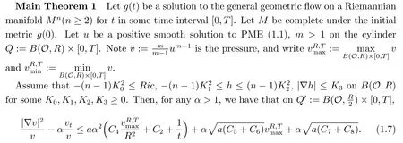
Ciis a constant depending onm,n,a,α,K0,K1,K2,K3,K4,R.

RemarkWhenh=−2Ric,(1.6)is the Ricci flow equation.In this case our results reduce to[8].Note that for Ricci flow the assumption|∇Ric|≤K3is not needed because of the contracted second Bianchi identity[[9],section 4].

As an application,we get the following result.

Corollary 1.1vis the pressure,then for anyx1,x2∈B(O,R/6)and anyα>1,

whereγ(s)is a smooth curve connectedx1andx2withγ(t1)=x1andγ(t2)=x2,|γ′(s)|sis the length of the vectorγ′(s)at times.

We extend the Laplacian operator to the drifting Laplacian operator,and we can get similar gradient estimate.

Main Theorem 2Let(Mn,g,dv)be a smooth metric measure space.Suppose thatuis a positive solution to(1.5).If|∇f|≤c0,|∇2v|≤c1,(Bp(2R))≥−k0,−k1≤h≤k2,|∇h|≤k3.Here,k0,k1,k2,k3≥0,then on the ballBp(R)we have

wherec2,c3,c4are constants depending ona,c0,c1,α,m,n,H,R,T,and

Corollary 2.1Let(Mn,g,dv)be a smooth metric measure space with|∇f|≤c0,|∇2v|≤c1,≥−k0,−k1≤h≤k2,|∇h|≤k3.Here,k0,k1,k2,k3≥0 suppose that(Mn,g)is a complete non-compact Riemannian manifold anduis a positive solution to(1.5),then

whereciis a constant depending ona,α,m,n,S,T,andS=

RemarkWhengis independent oft,our results reduce to[10].

2 Proof of Main Theorems

First,let us calculate a formula forL(Fα).

Lemma 2.1

Lemma 2.2 Letg(t)be a solution to the geometric flow on a Riemannian manifoldMn(n≥2)for t in some time interval[0,T].LetMbe complete under the initial metricg(0).Let u be a positive smooth solution to(1.1)on manifold(Mn,g(t))for somem>0,and letv:=be the pressure.Then we have

ProofCalculate directly by using the Lemma 2.1.

Proposition 2.1Letuandvbe as in Lemma 2.2.Then

ProofThe following formula is helpful in the calculation:

Using(2.6)and Lemma 2.2 we have

These give that

Using the formula

we have

Hence we obtain

Note the fourth to eighth terms in the above equation,they can be rewritten as

This completes the proof.

Then,we prove a local estimate for PME on complete manifolds under general geometric flow.We use the technique of Li and Yau[11]and some calculation of Lu,Ni,V´azquez and Villani in[3].Denote byB(O,R)the ball of radiusR>0 and centeredOin(Mn,g(t)),and denote byr(x,t)the distance function fromOtoxwith metricg(t).

Proof of the Main Theorem 1

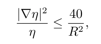
(i)Since boundedhtensor implies thatg(t)is uniform equivalence to the initial metricg(0)[[12],Corollary 6.11],that ise−2K1Tg(0)≤g(t)≤e2K2Tg(0).By definition,we know that(M,g(t))is also complete fort∈[0,T].Inspired by the choice of cutoff function in the proof of Theorem3.1 in[10],we letη(x,t):=θ(r(x,t)/R)be cutoff function,whereθ(s)is a smooth monotone function which satisfiesθ(s)≡1 for 0≤s≤1/2,θ(s)≡0 fors≥1,and(θ′)2/θ≤40,andθ′′≥−40θ≥−40.OnB(O,R),using the Laplacian comparison theorem,one can easily get

and

(ii)After the preparation in(i),now we applyLtotη(−Fα)and use the maximum principle to obtain our estimates.Iftη(−Fα)≤0 onQ,then the main theorem 1 is trivial.So we assume max(x,t)∈Qtη(−Fα)>0.Supposetη(−Fα)achieves its maximum at(x0,t0).Then we havet0>0 and

at(x0,t0).From now on,all calculations are at(x0,t0).

By the evolution formula of geodesic length under geometric flow(see[13]),we calculate

whereγt0is the geodesic connectingxandOunder the metricg(t0),Sis the unit tangent vector toγt0anddsis the element of arc length.

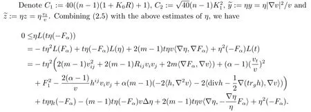
Here,we have used Proposition 2.1.Using the following inequality,(2.10)and(2.11)

we have

Using Young’s inequality,

and attention our assumption ofh,

On the other hand,

We get

Now writeC3:=80+C1and

Also note that

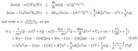
Using

then the above quadratical inequality(2.12)on(y−αz)reduces to

Proof of the Corollary 1.1Direct calculation implies

The result follows from the observation thatγ(s)lies completely insideB()at any time in[0,T](since bounded tensorhimplies thatg(t)is uniform equivalence to the initial metricg(0))and the estimate in the main theorem 1.

To prove the main theorem 2,we need some lemmas as well.Note

Suppose thatuis a positive solution to(2.13).Letv=.Direct calculation shows that

Since0,then(2.14)is equivalent to

LetL=∂t−(m−1)v∆fandF=.We have the following lemmas.

Lemma 2.3Suppose thatuis a poistive solution to(2.13).Then

ProofDirect calculation shows that

Therefore,we get

and

By(2.15)and Lemma 2.1,we have

According to(2.18),(2.19),(2.20),and(2.21).We conclude that

On the other hand,by(2.14)we get

Direct calculation shows that

According to(2.23)and(2.24),we obtain

According to[[14],[15]],we have

By(2.25)and(2.26),we conclude that(2.17)is true.

Lemma 2.4The functionFsatisfies the following equation:

ProofFor the reader’s convenience,we give the details of the proof of Lemma 2.4.By(2.16)and(2.17),we have

By the definition of F,we have

According to(2.15)we get

Using(2.15)again,we arrive at

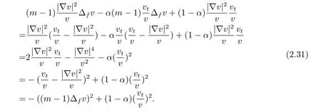
Putting(2.29),(2.30)and(2.31)into(2.28),we conclude that(2.27)is true.

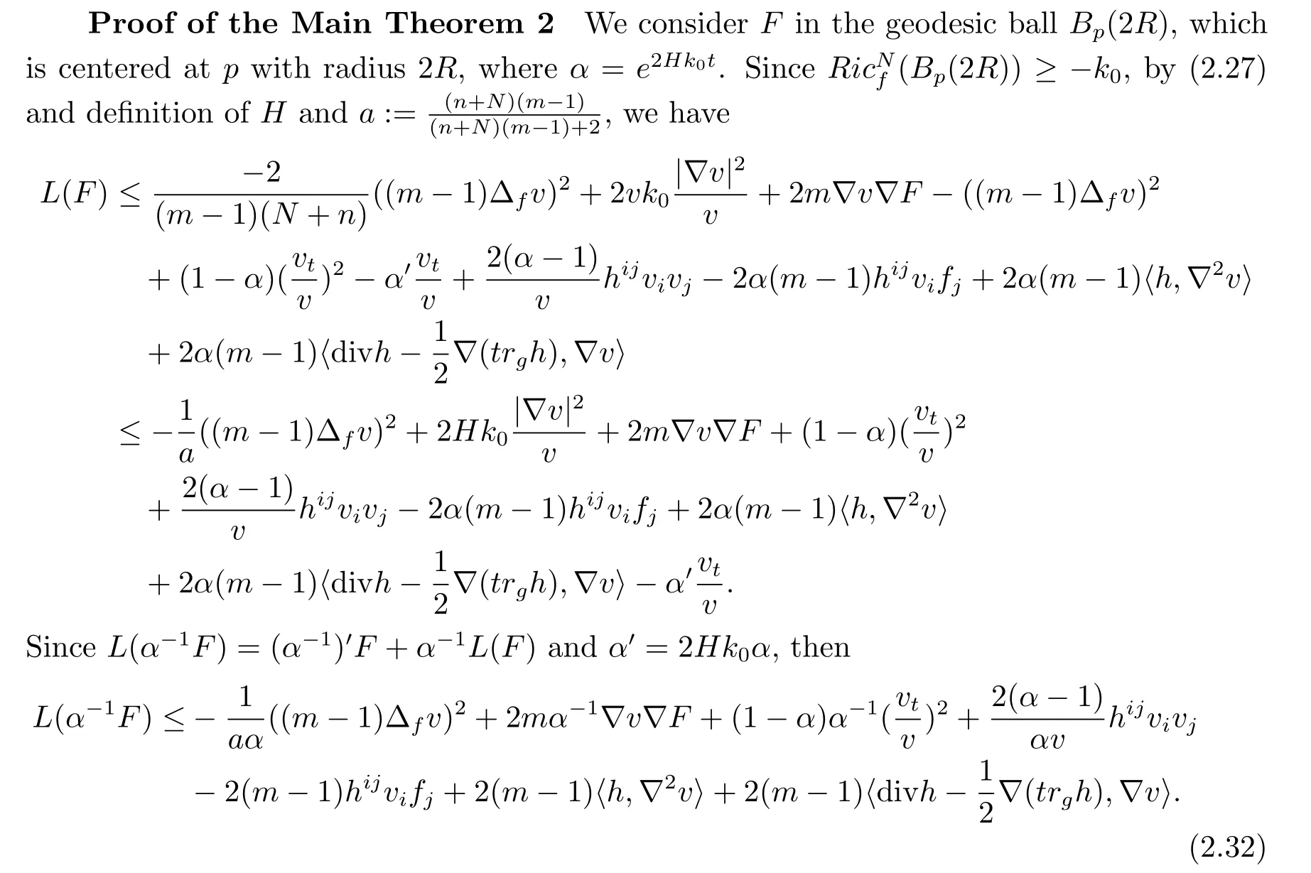
By(2.15)and definition ofF,we get

Putting(2.33)into(2.32),we obtain

Attention the definition ofh,|∇f|,the following reality and the Young’s inequality,

we have,

where we have used−ax2+bx≤b2/4ato the first term in the second inequality.

According to(2.4)and(2.5)in[7],we can construct a cut-off functionφsuch that 0≤φ≤1,sup(φ)⊂Bp(2R),φ|Bp(R)=1 and

whereCis a constant depending only on n.SetG=tφα−1F.Assume thatGachieves its maximum at the point(x0,s)∈Bp(2R)×[0,T]and assumeG(x0,s)≥0.By the maximum principle,we have

at the point(x0,s),and

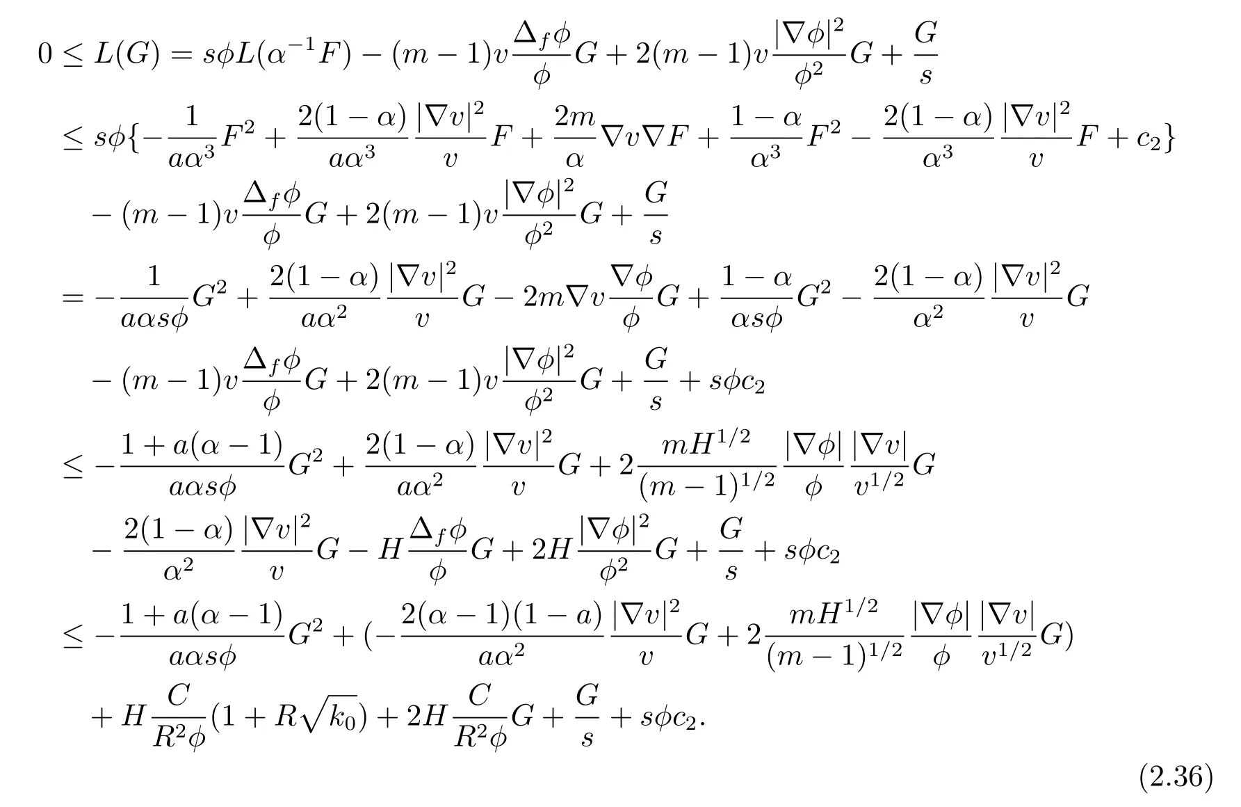
Multiplying both sides of(2.36)bysφ,and using−ax2+bx≤b2/4a,we get

inequality becomes

We can get

Hence,for allx∈Bp(R),it holds that

Thus,the proof of the main theorem 2 is completed.LettingR→∞,c4→,we get the result of Corollary 1.2.