随机时滞网络控制系统的后退时域估计
2020-06-11李超超韩春艳
李超超,韩春艳,何 芳
(济南大学自动化与电气工程学院,山东济南 250022)
1 Introduction
Recently,significant attention has been paid to networked control systems (NCSs)as they bring numerous benefits,such as reduced system wiring,lower cost in maintenance,increased system agility,ease of information sharing,etc.Along with the advantages,several challenging problems,such as bandwidth allocation,communication delays and packet dropouts,also emerged giving rise to many important research topics[1–4].Transmission delay is now well known to be one of the most often occurred phenomena in NCSs,which may result in deterioration of system performance and even instability.Therefore,it is of great significance to study NCSs with transmission delays where the packet dropout incorporates naturally.
There is no doubt that state estimation is an important topic in both theoretical research and practical applications.In the past decade,a substantial body of literature has been devoted to state estimation for systems with transmission delays.There existed several techniques for dealing with time delay,such as the classical state augmentation method[5],the linear matrix inequality algorithm[6],the polynomial approach[7],and the reorganization innovation analysis method[8].
The transmission delay in NCSs may vary with time and is often modeled as a random process.Two stochastic processes:the Bernoulli process[9–13]and the Markov process[14–15],are commonly used to describe the characteristics of the random delays.In [10],the recursive estimation for linear and nonlinear systems with uncertain observations were considered.A binary switching sequence-the Bernoulli distribution process,was used to describe the uncertainty in the observations.An estimator was obtained by the covariance information method.Similar result was also given in [11].In[14],the state estimation with missing measurements was considered,where the missing process was modeled as a Markov chain.A jump linear estimator was introduced to cope with the losses.Further in [12],an optimal filter problem with random delay and packet dropouts was studied,where the random received observations were stored in a possibly infinite-length buffer.In [13],the optimal and suboptimal linear estimators were designed for NCSs with random observation delays,where the random delay was modeled as a set of Bernoulli variables.The measurement reorganization method was employed for treating delay terms.In addition,the Markov type transmission delay was considered in[15]and three different types of filters were designed without state augmentation.
On the other hand,receding horizon estimation,also called moving horizon estimation,has become as an important research topic and gained much attention[16–19]in recent years.It explains the concept of full information estimation and introduces the moving horizon estimation as a computable approximation of full information.The basic design method for ensuring stability of moving horizon estimation was presented in [16].Further,the moving horizon estimation algorithm was applied to the field of distributed estimation in[17–18].In this paper,we will combine the receding horizon estimation algorithm and the observation reorganization technique to derive the estimator of the systems with random time delays,which reduce the calculation complexity for the design process.
Based on the aforementioned literature,we investigate the receding horizon estimation for discrete-time linear system with random observation delays.A set of Bernoulli variables are introduced to describe the characteristics of the random delay,and the measurement reorganization technique is employed for dealing with the delay terms.On the basis of the new system model without time-delay,both batch form and iterative form receding horizon estimation are derived afterward without state augmentation,and the stability analysis is supplied.
The contribution of this paper can be stated as:i)Compared with the Kalman-type estimator developed in[13],the receding horizon estimator developed in this paper,since based on a finite number of system measurements,can make more flexibility to tune weighting parameters and provide a higher estimator precision.The comparison has been shown in Section 4;ii)The Hadamard product is introduced in the derivation of the receding horizon estimator gains.This is the main difference between the receding horizon estimation developed in this paper and the Kalman-type estimator developed in[13];iii)In the derivation of estimator gains,it is difficult to solve a global optimization problem.Then the decomposition method is employed,by which the receding horizon estimation subject to unbiasedness constraint is divided intoNindividual optimization problems.The independent optimization problem is solved by the optimality principle,and the individual estimation gains are obtained.This is one of the technique contribution of this paper.
The remainder of this paper is organized as follows.Problem description is given in Section 2.Section 3 mainly concerns with the design of the receding horizon estimation and the stability analysis of the proposed method.In Section 4,a simulation example is presented to illustrate the estimator’s performance.Finally,conclusions are drawn in Section 5.
Notation:Throughout this paper,the superscripts−1andTrepresent the inverse and transpose of the matrix.represents the n-dimensional Euclidean space.Moreover,E{·}means the mathematical expectation,⊙is the Hadamard product,col{·}indicates the column vector,tr{·}means the trace of a matrix and P{·}represents the occurrence probability of an event.
2 Problem description
Consider the following discrete-time linear system with random delay:

wherex(t)∈is the state,w(t)∈is the input noise,yr(t)∈is the measurement andv(t)∈is the measurement noise.Through the paper,it is assumed that the constant matricesA,C,Hare known,[C,A]is observable,Ais nonsingular,andr(t)means the random delay.
Assumption 1w(t)andv(t)are white noises with covariance matrices E{w(t)wT(s)}=Qwδts,E{v(t)vT(s)}=Rvδts,respectively.x0,w(t),andv(t)are mutually independent.
Assumption 2Measurements in (2)are timestamped.As is well known,time-stamping of measurement information is necessary to reorder packets at the receiver side because there exist random delays in communication.The random delayr(t)is bounded with 0r(t)r,whereris known as the length of memory buffer.If the received measurement is with a delay larger thanr,it will be viewed as the lost packet.The probability distribution ofr(t)is P(r(t)=i)=ρi,i=0,…,r.Obviously,We assume thatr(t)is independent ofx0,w(t),andv(t).
Since formula (2)contains random delays which can’t be treated directly by the reorganized observation technique,the original system needs to be transformed into a constant delay one first.Based on the above assumption,denote

withαi,tdefined as a binary random variable indicating the arrival of the observation packet for statex(t −i)at timet,that is

Thenαi,t(i=0,1,…,r)has the same stochastic probability as that ofr(t).That means P(αi,t=1)=ρi(i=0,1,…,r),whereρi(i=0,1,…,r)is known.In the real-time control systems,the statex(t)can only be observed at most one time,and thus the following assumption needs to be made.
Assumption 3The stochastic variableαi,t(i=0,1,…,r)has the following property

Then the optimal filtering problem considered in this paper can be stated as follows:
Problem 1(Optimal receding horizon estimation)Given the observation{y(s)|0≤s≤t},find a linear minimum mean square error receding horizon estimator(t)of the statex(t)with the finite horizonN,such thatEw,v[(t)]=Ew,v[x(t)].
3 Construction of the receding horizon estimation
In this section,the random delayed system is transformed into a delay-free one by the reorganization observation method used for dealing with the random delay.Then,we will propose a new receding horizon estimator with deterministic gains by minimizing the mean square estimation error.
3.1 Observation reorganization
Because the state estimation for time-delay systems cannot be deduced directly,it needs to be transformed into a delay-free one by the reorganization observation method.
For the given timet,the received observations can be rearranged into a set of delay-free sequences as follows.


In addition,the covariance matrices ofvr(s)andvt−s(s)are described as follows:
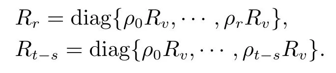
For convenience,denote

3.2 Receding horizon estimator
The problem considered here is how to acquire a receding horizon estimate(s|s −1)of the state vectorx(s)by using a finite number of measurements of the system output ¯y(s)with weighted matrix.And two forms of receding horizon estimation are derived from the following two theorems.
In order to simplify the calculation,let us define in Step 1 as
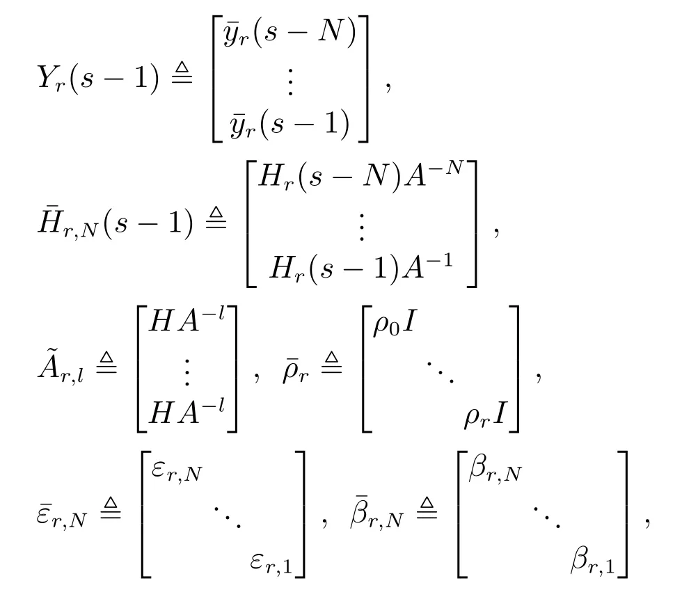

where⊙means Hadamard product andX(s)satisfies

It is noted that some definitions of the algorithm for Step 2 are similar to those definitions above,which just need to replace the subscriptrwitht −s,and thus is omitted here.
For the given timet,we now develop a batch form receding horizon estimator(t)in the following algorithm.
Algorithm 1(Batch form receding horizon estimator)
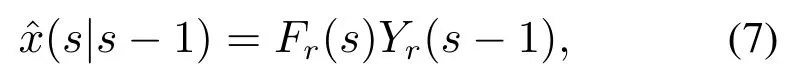
Step 1For 0st −r,a receding horizon estimator(s|s −1)is calculated by
where the optimal gain matrixFr(s)is determined by

with

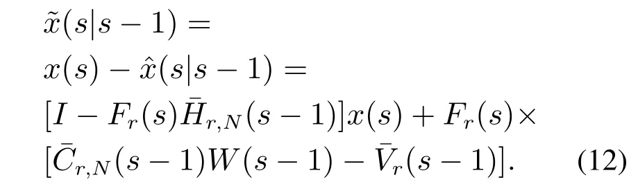
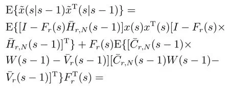
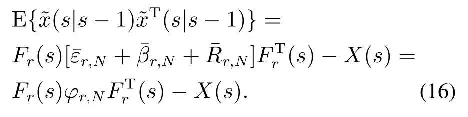
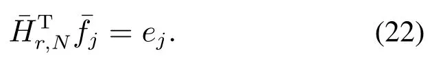
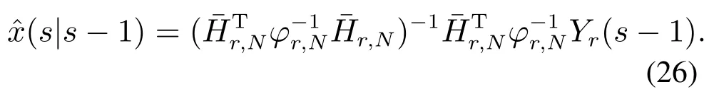
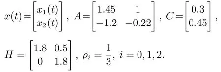
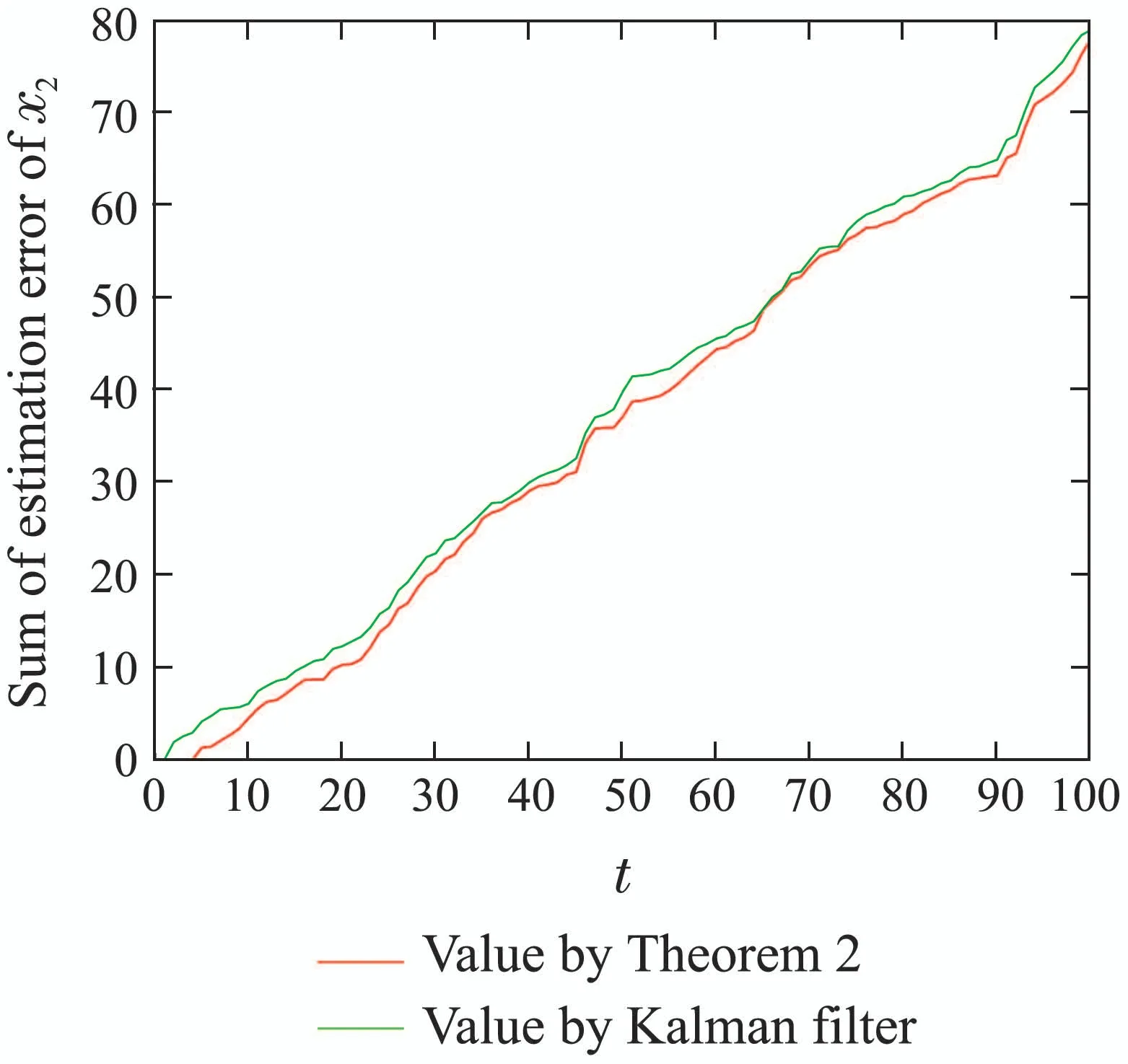
Step 2Fort −r Step 3Fors=t,set(t)=(t|t−1)in Step 2. In the following theorem,we will show that the estimator developed in Step 1–3 is the optimal solution to Problem 1. Theorem 1For systems (1)(4)and (5),when(C,A)is observable,the linear minimum mean square error receding horizon estimator(t)with a batch form on the horizon[t −N,t]can be derived by Algorithm 1,which satisfies the unbiased constraints. ProofFor 0st −r,the finite number of measurements on the horizon[s −N,s]can be expressed in terms of the statex(s), Taking expectation on both sides of(10),and to satisfy the unbiased condition,E=Ex,the following relation is obtained Based on the definition of estimation error,denote So,we can obtain the covariance of estimation error(s|s −1)as follows: By the foregoing definitions,the following results can be drawn: From(13)–(14)and(15),we obtain The objective is to obtain the optimal gain matrixF(s),subject to the unbiasedness constraint (11),in such a way that the error ˜x(s|s −1)of the estimate(s|s −1)has minimum variance as follows: Before obtaining the solution to(17),we obtain the result on constraint optimization in the first instance.In order to simplify the calculation,usingFrfor a temporary replacementFr(s).Now,suppose that the following trace optimization problem is given For convenience,partition the matrixFrin(11)as From(19),as a consequence,thes-th unbiasedness constraint can be written as In terms of the partitioned vector,the cost function(18)is represented as Thus,the optimization problem (18)is reduced toNindependent optimization problems subject to Obtaining the solutions to each optimization problem (21)and putting them together,we can finally obtain the solution to(17). By solving the optimization problem (21),we can firstly establish the cost function whereλjis thes-th vector of a Lagrange multiplier,which is associated with thes-th unbiased constraint. In order to minimizeΦ,two necessary conditions are obtained Putting them together,we can obtain Bring(25)into(10),we can reach the batch form of receding horizon estimation The derivation of Step 2 is similar to that of Step 1.This completes the proof of Theorem 1.QED. Remark 1In the derivation of Theorem 1,the linear minimum mean square error receding horizon estimation subject to unbiasedness constraint is divided intoNindividual optimization problems.Then,by introducing the Lagrange multiplier,the independent optimization problem is solved,and the individual estimation gains are obtained.At last,the total gain is obtained by putting all the components together.The amount of computation meets our requirements.In addition,in(17),Fr(s)should be updated over time. In what follows,we will rewrite the batch form estimator in an iterative form for computational advantage.For the given timet,an iterative form receding horizon estimator(t)is developed. Algorithm 2(Iterative form receding horizon estimator) Step 1For 0st −r,an iterative form estimator(s|s −1)with finite horizonNis given by where Step 2Fort −r Step 3Fors=t,set(t)=(t|t−1)in Step 2. It will be shown in Theorem 2 that the iterative estimator developed in Algorithm 2 is the optimal solution to Problem 1 subject to unbiased constraints. Theorem 2Assume that (C,A)is observable.Then the linear minimum mean square error receding horizon estimator(t)with an iterative form on the horizon[t −N,t]is given by Algorithm 2,which satisfies the unbiased constraints. ProofFirstly,for 0st −r,define So it can be represented in the following Riccati Equation for 0lN: Similarly,it is available for 0lNthat From (28)and (29),an iterative form for receding horizon estimation is obtained Similarly,We are able to get an iterative form of receding horizon estimation in Step 2.This completes the proof of Theorem 2.QED. The stability of the receding-horizon estimator will be investigated below.Thus we just need to analyze the stability of the filter developed in Theorem 2.It needs to require consideration of the filter’s transfer matrix.From Theorem 2,we define the transfer matrix for 0st −ras Under the given assumption,the necessary and sufficient condition subject to asymptotical stability of the proposed filter is that the transfer matrixΓNof the estimator is one stability matrix.It means that all of its eigenvalues are located in the unit circle.The stability of the observer is ensured by the following theorem. Theorem 3If(C,A)is observable,andAnonsingular,then the matrixΓNhas all its eigenvalues strictly within the unit circle for all finiteNn −1 wherenis the dimension of the state vector. ProofFor 0st −r,define[20] In view of(28)and(29),we can obtain(30)immediately.This completes the proof of Theorem 3.QED. Remark 2Conditions for the stability of the proposed moving horizon estimation is proposed for time-invariant systems.The advantage of this estimation algorithm is that it is easy to implement since the gains can be performed off-line. In this section,a simulation example is given to illustrate the efficiency of the proposed receding horizon estimation for random delay system(1)and(2).In this part,we define the time horizon 0t100,the estimator horizon sizeN=5,and the random delay horizon 0r(t)2.The other parameters of the system are as follows Fig.1 State trajectories of x1(t) Based on the design procedures of Theorem 2 in this paper and Kalman filter in [13],the simulation results are obtained as follows.Fig.1 shows the trace of the real valuex1(t)and its estimate.Fig.2 shows the trace of the real valuex2(t)and its estimate.Fig.3 shows the root of the mean square estimation errors(RMSEEs)ofx1(t)according to the two algorithms,while Fig.4 shows the RMSEEs ofx2(t)according to the two algorithms.Fig.5 shows the summation of the RMSEEs ofx1(t)of the two algorithms.Fig.6 shows the summation of the RMSEEs ofx2(t)of the two algorithms.It can be seen from Figs.3–6 that the obtained receding horizon estimation for systems with observation delays track better than Kalman filter and the estimation scheme produces better performance.On the other hand,it can be seen from Fig.7 and Fig.8 that the tracking performance for the case ofN=5 is better than that ofN=2.It is a suitable choice for the estimator horizon sizeN=5. Fig.2 State trajectories of x2(t) Fig.3 The RMSEEs of x1(t) Fig.4 The RMSEEs of x2(t) Fig.5 Summation of RMSEE trajectories of x1(t) Fig.6 Summation of RMSEE trajectories of x2(t) Fig.7 Summation of RMSEE trajectories of x1(t)for RHE estimation: N=5,2 Fig.8 Summation of RMSEE trajectories of x2(t)for RHE estimation: N=5,2 In this paper,the receding horizon estimators were proposed for discrete-time linear system with random observation delay.The random delay system was transformed into a delay-free one by the reorganization observation method.On the basis of the new observation equation,a batch form and an iterative form for receding horizon estimation were designed.The observation reorganization technique is firstly applied to the receding horizon estimation for discretetime systems with random delays.It is obvious that this method simplifies the computation compared to state augmentation method for dealing with random delays.This is the main technique novelty of this paper.The stability analysis was supplied and the theoretical results were illustrated by a numerical example.


3.3 Stability analysis


4 Simulation example


5 Conclusion