Variable slip window technology in transition detection on pitching airfoil
2020-06-11BinbinWEIYongweiGAODongLILeiDENG
Binbin WEI, Yongwei GAO, Dong LI, Lei DENG
School of Aeronautics, Northwestern Polytechnical University, Xi’an 710072, China
KEYWORDS Data processing;Dynamic characteristics;Pitching airfoil;Transition and relaminarization;Variable slip window technology (VSWT)
Abstract In the pitching motion, the unsteady transition and relaminarization position plays an important role in the dynamic characteristics of the airfoil. In order to facilitate the computer to automatically and accurately calculate the position of the transition and relaminarization, a Variable Slip Window Technology (VSWT)suitable for airfoil dynamic data processing was developed using the S809 airfoil experimental data in this paper and two calculation strategies, i.e., global strategy and single point strategy,were proposed:global strategy and single point strategy.The core of the VSWT is the selection of the window function h and the parameters setting in the h function.The effect of the VSWT was evaluated using the dimensionless pulse strength value (INB), which can be used to evaluate the signal characteristics,of the root mean square(RMS)value of the fluctuating pressure. It is found that: the h function characteristics have a significant influence on the VSWT. The suitable functions are Hn function constructed in this paper and step function. For the left boundary of the magnified area, the step function can obtain the largest INB value, but the robustness is not good. The H1 function (Gaussian-like function, n=1) can show higher robustness while ensuring a large INB value. The two computing strategies, which are single point strategy and global strategy, have their own advantages and disadvantages. The former strategy,that is the single point strategy, can achieve a higher INB value, but the RMS magnification at the feature position needs to be known in advance. Although the INB value obtained by the latter strategy,that is the global strategy,is slightly smaller than the calculation results of the former strategy, it is not necessary to know the RMS magnification at the feature position in advance. So the global strategy has better robustness.The experimental data of NACA0012 airfoil was used to further validate the developed VSWT in this paper,and the results show that the VSWT developed in this paper can still double the INB value of the transition/relaminarization position. The VSWT developed in this paper has certain practicability,which is convenient for the computer to automatically determine the transition/relaminarization characteristics.
1. Introduction
The unsteady characteristics in pitching airfoil should be carefully investigated due to its important impacts on wind turbines, helicopter rotor blades, jet engine compressor blades etc.However,the current airfoil design methodologies still rely on steady design criteria.1It is necessary to take into account the unsteady characteristics of the airfoil in the design of the airfoil.
During the pitching motion of the airfoil, the unsteady transition and relaminarization characteristics of the airfoil are often expected to be captured accurately.During the transition and relaminarization of the boundary layer, many features become apparent and observable, such as the increase of the thickness, surface temperature, wall shear stress and total pressure etc. in the boundary layer. Taking into account the ambiguity of the position of the transition and relaminarization, it is convenient to define the peak of the Root Mean Square (RMS) of temperature or pressure as the indication of flow transition and relaminarization.
In order to capture the unsteady characteristics in pitching airfoil, semi-empirical models, Computational Fluid Dynamic(CFD) method and experimental methods are often used.
The semi-empirical models have distinct characteristics.The semi-empirical models2can quickly calculate the aerodynamic characteristics of the airfoil under dynamic stall conditions. Therefore, the use of semi-empirical models to solve unsteady aerodynamic loads still dominates in the field of wind turbine aerodynamic design. However, semi-empirical models often lack a deep understanding of the real physical mechanisms3and they generally do not consider the hysteresis effect of transition.In addition,the maximum lift coefficient and the corresponding moment coefficient of the airfoil in the state of deep stall calculated by the semi-empirical models are significantly different from the experimental data.4
The CFD method is also a commonly used method for calculating the unsteady characteristics in pitching airfoil. The common practice is unsteady numerical calculation based on the RANS equation5-8. With the development of computers,the current CFD method can simulate the dynamic stall characteristics of the airfoil,but the amount of calculation is large.9In addition,it reduces the reliability of numerical results due to the use of static transition prediction model and semi-empirical dynamic stall model.At present,the CFD method is still difficult to calculate the unsteady transition characteristics.
At present, the more convincing method of capturing the unsteady characteristics in pitching airfoil is still the experimental method.In 1996,Pascazio et al.10studied the boundary layer transition and separation in pitching airfoils using the Embedded Laser Velocimetry (ELV) method. The research showed that the turbulent boundary layer behavior was modified by the transition delay.In 2016,Wang and Zhao11studied the development of the leading edge vortex under different dynamic stall conditions using the advanced Particle Image Velocimetry (PIV). They found that the development of the leading edge vortex was influenced by the leading edge radius,the angle of attack, the mean pitch angle and the oscillation frequency.
Currently,the airfoil dynamic characteristics are often captured by static airfoil experimental technique,such as fluctuating pressure methods,12-14hot wire method,15,16temperature sensitive paints method,17infrared thermography18and flow visualization methods11and so on. Unsteady characteristics in pitching airfoil are then obtained by calculating the features at different times,such as the RMS of the fluctuating pressure or temperature.
Researchers tend to average data over many cycles at the same phase to obtain the unsteady characteristics over a full cycle.The phase average method does not require a high sampling frequency to obtain the unsteady characteristics of the airfoil, but requires a very long sampling time.12In order to save time costs, we have developed the Slip Window Technology(SWT)to calculate the unsteady characteristics in pitching airfoil.13
The SWT solves the disadvantage that the sampling time of the phase average method is too long.In theory,the SWT only needs to acquire the fluctuating pressure data of an oscillation period to capture the unsteady characteristics of the airfoil.However, there are still two shortcomings in the SWT: (A)in a complete cycle, the transition/relaminarization characteristics are not obvious enough due to the extremely strong characteristics of flow separation and reattachment, which brings difficulties to automatically and accurately discrimination;(B) the accuracy of angle of attack at the feature position is not high enough.
In order to solve these two shortcomings in the SWT, a Variable Slip Window Technology (VSWT) was developed in this paper. And two computing strategies, ie. Global strategy(G VSWT) and Single Point strategy (SP VSWT), were proposed. The core of the VSWT is the selection of the window function h and the parameters setting in the h function.Calculation was made using fluctuating pressure of different airfoils and the effectiveness of the VSWT was verified. The calculation results showed that the VSWT developed in this paper is convenient for the computer to automatically and accurately calculate the position of transition and relaminarization.
2. Variable slip window technology
A SWT developed in our paper13has been used to process the fluctuating pressure data on the dynamic airfoil. However, there are still two defects in the SWT: (A) the characteristics of the transition and relaminarization are not obvious due to the large pressure fluctuation in the separation zone,and human judgment is required; (B) the accuracy of the angle of attack at the feature locations is not high enough.Therefore, a VSWT is developed aiming at avoiding the two defects.
The RMS value of the fluctuating pressure was calculated using13:
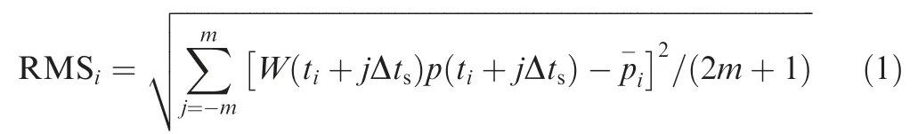
where W(t) is symmetrical window function, Δtsis sampling period, 2m+1 is window width.
The window function W(t)in Eq.(1)is rectangular window.Its window height and width do not change over time.On this basis, we hope to construct a variable rectangular window as shown in:

The window function and the window width change law is controlled by:

where m is the half window width,m0is the reference half window width value.
The shape of the window function h is described by:
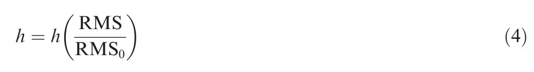
where RMS is the RMS value calculated in the window,RMS0is the reference value.
The angle of attack error in the window can be calculated by13:

where fsis the sampling frequency, f is the oscillation frequency,A is the amplitude and Δαsis the variation of α caused by discrete sampling with frequency fs.
The window height variation function h is hoped to possess the following properties: h increases as RMS/RMS0increases when RMS/RMS0<μ0; h takes its maximum value when RMS/RMS0=μ0; and h decreases as RMS/RMS0increases when RMS/RMS0>μ0.In addition,h has the minimum value controlled by Eqs. (3) and (4) due to that the half window width cannot be infinite.
Taking into account these properties of the h function, a window height variation function, Gaussian-like function, is constructed as follows:
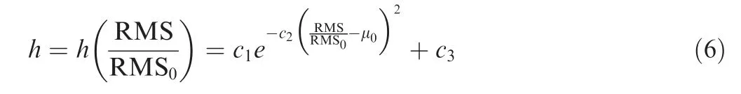
where c1is the amplification factor of the window height variation function h,c2is the shape factor,μ0is the threshold value of RMS/RMS0, c3is the offset coefficient.
The maximum value of h is c1+c3once the threshold μ0is determined.If c1+c3>1,the RMS value in the window will be larger than that in the paper13at the position of the threshold μ0, which can play a role in enhancing features. The half window width m will decrease due to the increase of h controlled by the Eq. (3), which can decrease the error of angle of attack controlled by the Eq.(5).Thus,the variable slip window W constructed in this paper makes up for the two shortcomings mentioned above in the SWT.
The realization process of the VSWT developed in this paper is as follows:
Step 1. Select parameters of m0, RMS0, c1, c2, c3and μ0.
Step 2.Calculate the RMS value of the fluctuating pressure using the reference half window width m0according to the SWT.
Step 3. Calculate the RMS/RMS0, and calculate the new window height h using Eq. (6).
Step 4. Calculate the new half window width m and round up,and then recalculate the new window height h using Eq.(6).
Step 5. Calculate the new weighted RMS value using the new window function W.
3. Discussion
The impacts of the h function on the results will be discussed in details in this section.
In this section, the experimental data of S809 airfoil is used. The test status can be found in article.13In this case, the model chord length was c=500 mm, the Reynolds number was.Re=0.75×10⁶, the oscillation frequency was f=0.5 Hz, and the reduced frequency was k=2πfc/U∞=0.0785.
3.1. Processing results of Gaussian-like curve
Firstly, the parameters of the Gaussian-like curve should be confirmed.
For the reference half window width m0: the dimensionless half window width determined in paper13is m-=0.0015 which can be used to calculate the m0.
For the offset coefficient c3: c3is the minimum value of h function and represents the maximum value of the half window width. The maximum half window width is set to mmax=m0in this paper, which will make hmin=m0/mmax=1, so c3is taken as c3=hmin=1.
For the amplification factor c1: the maximum value of h function is c1+c3. The c1is taken as c1=3 considering that the window height cannot be excessively large. (If the window height is excessively large,the window width will be excessively small according to Eq. (3). In practical applications, the window width cannot be less than 1.)
For the shape factor c2:it affects the change rate of the window height. Its impacts are studied in details in this paper which can be seen in Section 3.2 and Section 3.3. In general,c2can be taken as c2=1.
For the reference value RMS0: it can be selected as the RMS value of the sensor in the zero state of the wind tunnel.
For the threshold μ0: it is chosen according to different experimental conditions and purposes. The features at the transition/relaminarization are hoped to be highlighted in thispaper,so we choose the ratio of RMS value to the RMS0at the transition/relaminarization as μ0.
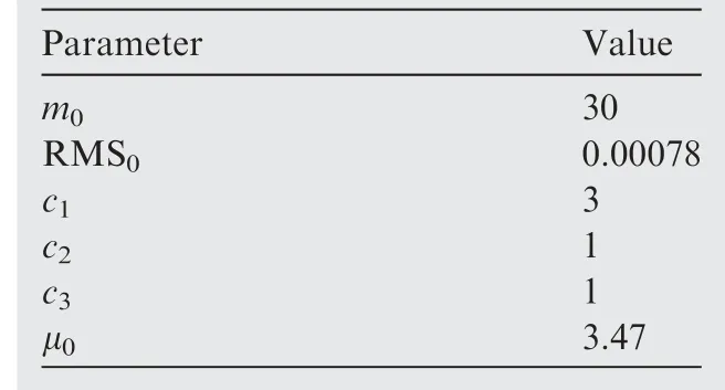
Table 1 Selections of parameter.

Fig. 1 Shape of window height variation function h.
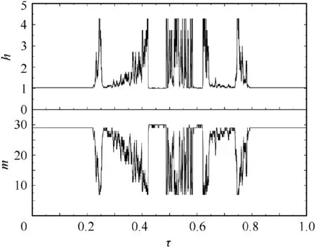
Fig. 2 Window function and window width curves.
The parameters during the calculation of the fluctuating pressure RMS are selected as shown in Table 1 in the case where the pressure measurement point is x=50 mm. The shape of the window height variation function h is as shown in Fig. 1.
Fig. 2 is the curve of window height and width in a complete cycle.The horizontal ordinate τ is the dimensionless time normalized by the oscillation period T:τ=t/T.It can be seen that the window height increases and will increase the RMS value when the transition/relaminarization occurs.Meanwhile,the window width decreases and will reduce the angle of attack error.
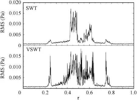
Fig. 3 Comparison of results of two technologies.
The results of the SWT and the VSWT are shown in Fig.3.It can be seen that the RMS value processed using VSWT increased significantly compared to that processed using SWT.
The dimensionless pulse strength (INB) defined in paper13is still used to evaluate the signal characteristics in this paper.The deleted neighborhood is chosen to be 1000 points.The calculation formula of INB is as follows:

where RMSNis the mean RMS value of the deleted neighborhood at time i,N is the neighborhood size which is N=1000.
Comparison of the INB values of the two different technologies of the SWT and the VSWT at transition/relaminarization is shown in Table 2. It can be seen that the INB value obtained by the VSWT increases in quantity compared to that obtained by the SWT at the two feature positions.
The error of angle of attack Δα was calculated using Δα=4mπAf/fscos(2πft) presented in Ref. 13. We compare the angle of attack error of the two different technologies of the SWT with the VSWT at transition/relaminarization as shown in Fig. 4. It can be seen that the angle of attack error Δα obtained by the VSWT reduced significantly at the two feature positions caused by the window width reduction in Fig.2.The parameter m is a constant in SWT,so Δα is a cosine function of time t. Whereas, the parameter m is also a function of time t in VSWT as shown in Fig.2,so the drastic change of m will lead to the change of Δα as shown in Fig. 4.
Comparison of Δα of the two different technologies of the SWT and the VSWT at transition/relaminarization is shown in Table 3. It can be seen that the Δα obtained by the VSWT decreases in magnitude compared to that obtained by the SWT at the two feature positions.
3.2. Effect of shape factor on results
The window function is the core in the VSWT developed in this paper. In the h function, the amplification factor c1, the offset coefficient c3, the threshold μ0and the reference value RMS0have more intuitive effects on the results, whereas, the effects of the shape factor c2on the results require in-depth study.
The h function curves for different c2cases are shown in Fig.5.The h function curve constructed in this paper is similar to the Gaussian curve,and gradually becomes‘thin and tall’as c2increases.Next,the effects of c2on the processing results are studied in this paper.
The fluctuating pressure data of the S809 airfoil with the reduced frequency of k=0.0785 at x=50 mm is still used as an example to illustrate in this section.
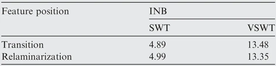
Table 2 INB value at the feature position.
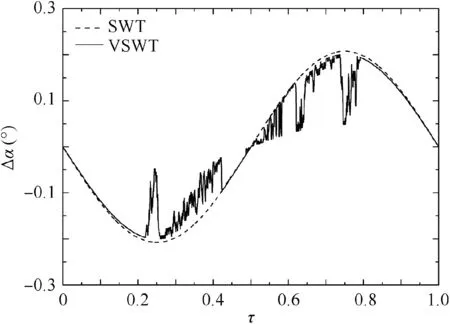
Fig. 4 Comparison of error of angle of attack between two technologies.

Table 3 Error of angle of attack Δα at the feature position.

Fig. 5 Effects of shape factor c2 on shape of h function.
The effects of the c2on the processing results are shown in Fig. 6. It can be seen that the RMS value at the location of transition/relaminarization is almost unchanged as c2gradually increases. However, the RMS values of its neighboring time are suppressed, which will increase the INB value at the position of transition/relaminarization.
The curves of the effect of the c2on the INB value at the position of transition/relaminarization are shown in Fig. 7. It can be seen that the INB value at the position of transition/relaminarization increases gradually as c2increases. The growth rate of INB value is relatively larger at 0.5 ≤c2<1.5 than that at c2≥1.5.
As shown in Fig. 5, the value at the symmetrical axis in h function is not affected by c2, so the height h and width m of the window function W at RMS/RMS0=μ0is not affected by c2, And the width m is a function of Δα, so the Δα at RMS/RMS0=μ0is not affected by c2, In this case, the RMS/RMS0at transition is RMS/RMS0=3.47=μ0, so the change of c2does not affect its Δα. And the RMS/RMS0at relaminarization is RMS/RMS0≈3.47=μ0, so the change of c2has a little affect on the Δα.

Fig. 6 Effects of c2 on processing results.
3.3. Two calculation strategies
The value of amplification factor c1, offset coefficient c3and the reference value RMS0determined in Section 3.1 can be used under different experimental conditions. However, the shape factor c2and threshold μ0vary depending on the experimental conditions.
Two strategies for the selection of the c2and μ0are proposed in this paper:(A)global strategy(G VSWT)considering all pressure points on the airfoil surface;(B)single point strategy (SP VSWT) for each airfoil pressure point.
The fluctuating pressure data on the S809 airfoil surface with a reduced frequency of k=0.0785, k=0.1571, and k=0.2356 presented in article13is still used as an example to illustrate.
3.3.1. Global strategy
The global strategy is designed to perform data processing on the data collected by all sensors on the airfoil surface using a set of parameters. The global robustness of the algorithm is first studied in order to ensure that the selected parameters have the desired effect on the data collected by all sensors.

Fig. 7 Effects of c2 on the INB value.
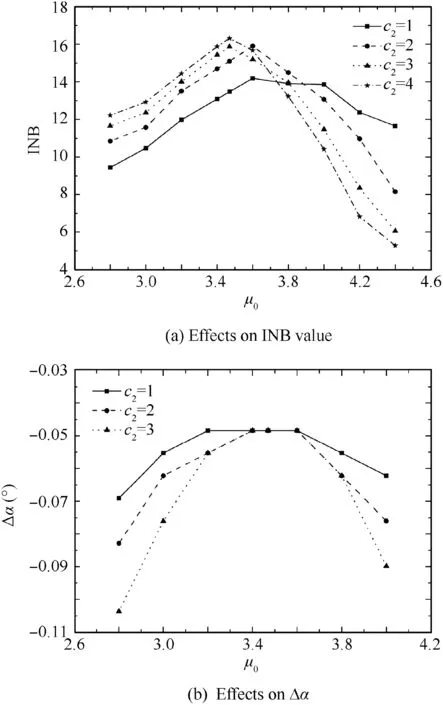
Fig. 8 Effects of μ0 at transition in different cases of c2.
The effects of μ0on the transition and relaminarization at the position of x=50 mm in the case of different c2are shown in Figs.8 and 9 including the effects on the INB value and Δα.
It can be seen that the μ0-INB curves have maximum in the case of different c2. When μ0exceeds μ0corresponding to the maximum of INB, the value of INB will decrease, whereas,the decay rate varies with c2. When c2is large, the INB will continue to decay rapidly.The value of INB will decay rapidly to INB≈5 when c2=3,4 at transition as shown in Fig. 8.Note that in Table 2, the processing result of SWT for transition is INB=4.89. It can be seen that when c2=3,4, the result obtained by VSWT is not better than that by SWT in the case of μ0=4.4.
That is to say,the INB value at the feature position is more sensitive to the change of μ0when the value of c2is too large,which will result in that the small difference between different sensors may result in significantly different INB value.
In addition, it can be seen from the μ0-Δα curves that the error of angle of attack Δα have minimum at transition and relaminarization in the case of different c2. The μ0-Δα curves have the same extreme point in the case of different c2. Also,μ0has little effect on Δα near the extreme point, while μ0has a large effect on Δα in areas far from extreme point. In areas far from extreme point,Δα will increase sharply as c2increases.

Fig. 9 Effects of μ0 at relaminarization in different cases of c2.
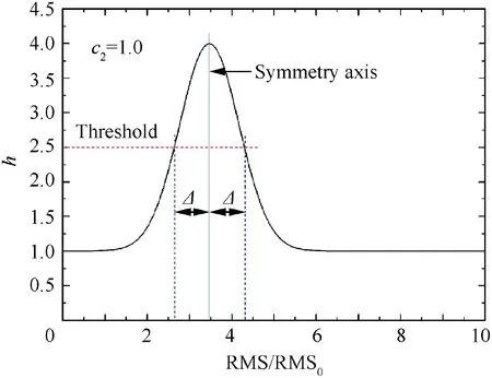
Fig. 10 Schematic diagram of calculation of magnified area Δ.
The amplifiable area is used to measure the robustness of the VSWT in this paper. A schematic diagram of the calculation of the amplifiable area Δ is shown in Fig. 10. Take c2=1.0 as an example. For such an h function curve, select the threshold for h first and record it as th. Calculate the abscissas of the left and right points when h ≥th, and record them as xland xr.The axis of symmetry of the h function curve is RMS/RMS0=μ0. Thus, the calculation formula of the amplifiable area Δ is Δ=μ0-xlor Δ=xr-μ0. In the interval RMS/RMS0∈[μ0-Δ,μ0+Δ], the signal can obtain the magnification of h ≥th. The size of the amplifiable area Δ can directly measure the size of the effective region where the magnification at least th can be obtained.And the size of this effective region directly determine the robustness of the algorithm.
The curves of Δ versus c2for different thresholds th are shown in Fig. 11. It can be seen that the amplifiable area decreases sharply as c2increases which will cause the robustness of the algorithm to drastically deteriorate.

Fig. 11 Δ curves with c2.
The experimental data of the S809 airfoil with the reduced frequency of k=0.0785, k=0.1571 and k=0.2356 will be used as follows. The ratio of the RMS at the feature position to the RMS value of the zero state at the corresponding position has been statistical in this paper.
The ratio of the RMS at the feature position transition/relaminarization is shown in Fig. 12. The red dot line in the figure is the mean value of the ratio corresponding to μ0in the h function and the blue dot line is the boundary that covers most of the points. The area between the red dot line and the blue dot line corresponds to the amplifiable area Δ introduced previously.
Fig.13 is the variation of the mean value μ0and amplifiable area Δ with reduced frequency in Fig.12.It can be found that the mean value μ0and the amplifiable area Δ increases sharply as the reduced frequency gradually increases to k=0.1571.
A specific reduced frequency corresponds to a specific amplifiable area. It can be seen from Fig. 11 that a specific c2value is corresponding to the amplifiable area for a specific growth rate case. This value is the maximum of c2under the condition of ensuring the robustness of the algorithm. Once c2exceeds this value, the algorithm will not guarantee that the RMS value at all pressure points on the airfoil can be amplified.
In addition,it can be seen from Fig.11 that the enlargement of the amplifiable area Δ will cause c2to decrease in the case of a certain rate of increase. Therefore, as can be seen from Fig. 13, the maximum value of c2that guarantees the robustness of the algorithm will decrease sharply with the increases of the reduced frequency.
It can be seen that the effect of c2on the INB value and the robustness of the algorithm is reversed under the parameter selection criteria of the global strategy. The pursuit of a large INB value will inevitably lead to the instability of the algorithm. In fact, Fig. 7 shows that the algorithm can still obtain an ideal INB value when c2is small.Therefore,we can choose a suitable small c2to balance the INB value and algorithm robustness.
We hope to improve the INB value as much as possible while ensuring the robustness of the algorithm. In this case,the suggested values of μ0and c2in the h function at th=2.0 and the corresponding amplifiable area Δ are given in this paper as shown in Table 4.

Fig. 12 Ratio of RMS at feature position.
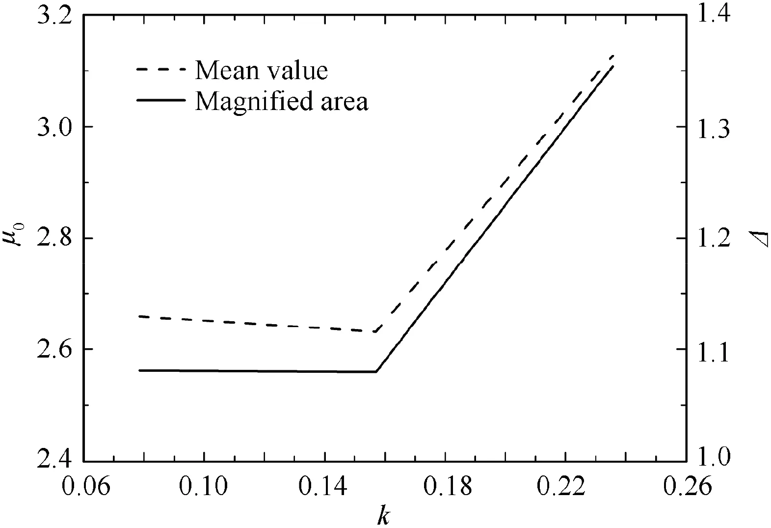
Fig. 13 μ0 and Δ curves with the reduced frequency.
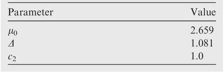
Table 4 Suggested values of parameters with reduced frequency k=0.0785.
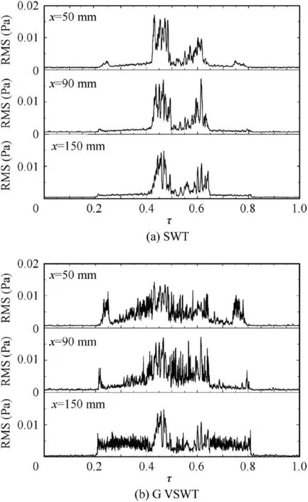
Fig. 14 Calculation result of global strategy with the reduced frequency of k=0.0785.
The experimental state with the reduced frequency of k=0.0785 is calculated using the global parameters determined in Table 4. Fig. 14 is a comparison of the calculation results of the two methods with the reduced frequency of k=0.0785.Take the results at three typical locations for comparison.It can be seen that the calculation results using VSWT are significantly improved compared to that using SWT. It should be noted that the parameters determined by the global strategy guarantee the robustness of the algorithm over the entire airfoil surface, but they do not guarantee that a very large INB value can be obtained for each position. Even so,the results obtained by the VSWT are still significantly better than that obtained by the SWT with such parameters.
3.3.2. Single point strategy
The parameters determined by the global strategy guarantee the validity of the parameters over the entire airfoil surface,but they do not guarantee an optimal choice for each sensor.Regardless of the global parameters versatility, different combinations of parameters(c2and μ0)can be taken for each pressure point location.
According to Fig. 12, the RMS magnification of transition and relaminarization at each position is taken as the mean value μ0.In the single point strategy,the parameter c2is taken as c2=8.0 to ensure a sufficient large INB value.
Fig. 15 is the calculation result using the single point strategy with the reduced frequency of k=0.0785.Comparing the results of the global strategy in Fig. 14, it can be seen that the features of the results using single point strategy are more obvious.
3.3.3. Comparison of results of two strategies
In order to quantify the calculation results of the two strategies, the INB value and the error of angle of attack Δα of the results of different strategies are calculated in this paper.
The INB value of different calculation strategies in the case of k=0.0785 is shown in Fig.16(a).Among them,the results of the SWT are represented using black color;the results of the G VSWT are represented using red color and the results of the SP VSWT are represented using blue color. In addition,the solid pattern represents the calculation results of the transition and the hollow pattern represents the calculation results of the relaminarization. It can be seen that the INB value calculated by the VSWT developed in this paper is obviously improved compared with the results obtained by the SWT.And the INB value has an increase in magnitude in some places.
The error of angle of attack Δα of different calculation strategies are shown in Fig.16(a)and Fig.16(b).It can be seen that the Δα of G VSWT and SP VSWT are all significantly reduced compared with that of SWT.
We develop two implementation strategies for VSWT: global strategy and single point strategy.Fig.16(a)shows that the SP VSWT yields a larger INB value than the G VSWT. However,the SP VSWT requires prior knowledge of the RMS magnification at the transition/relaminarization(compared to zero state).If the magnification at the transition/relaminarization is already known, the significance of the implementation of the VSWT developed in this paper will be reduced.
In the case of not seeking excessively large INB value, the RMS magnification does not need to be known in advance using the G VSWT developed in this paper and we only need to determine a rough range. As can be seen from Fig. 16, the INB value is doubled and the Δα is greatly reduced at the feature position under such a global strategy.This ensures that a large INB value can be obtained and the actual implementation of the algorithm is guaranteed.

Fig. 15 Calculation result of single point strategy with reduced frequency of k=0.0785.
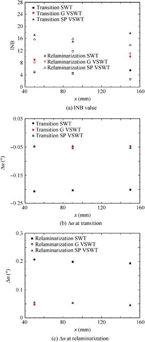
Fig. 16 INB value and error of angle of attack Δα of different strategies in case of k=0.0785.
3.4. Discussion of h function optimization
We construct an h function in the form of a Gaussian-like curve. In fact, there are many functions that can be used as the h function in the VSWT developed in this paper. A class of h functions is constructed in this section. Based on these h functions, we attempt to discuss its optimal properties: what conditions do the h function satisfy when the optimal calculation results are obtained in the case of a amplification threshold th.
A class of h functions constructed in this section is as follows:

The parameters in the formula are consistent with the parameters in Eq. (6). When n=1, the function is the Gaussian-like function in the previous text.
The Hnfunction without considering the translation amount are shown in Fig. 17. The parameters in the Gaussian-like function are: c1=3, c2=1.0, μ0=3.5,c3=1.0. Δ is the magnified area when th=2.0 (without considering the translation amount, th=1.0). The left and right borders of the magnified area are pland prrespectively. In the Hnfunction, c1=3, μ0=3.5, c3=1.0, and c2depends on the magnified area determined by the Hnfunction. It can be seen that the limit of this class of function is a step function.
In Fig. 17, the wine dotted line is the axis of symmetry of the Hnfunction. As n gradually increases, the Hnfunction gradually approaches the step function. On the left side of the point pl,Hnhas no amplification effect on the RMS value.Once the point plis crossed, the amplification amount is abruptly changed to the maximum value,so that the INB value at point plis the largest.
Define the cumulative function as follows:

Fig.18 is the cumulative function of Hnfunction.To quantitatively describe the role of the Hnfunction, the slope of the cumulative function is defined as follows:

The larger the K value,the closer the Hncurve is to the step function.It is easy to get that the slope of the cumulative function of step function is K=1/ (2 Δ). And this K value is the maximum K value in a certain magnified area.
The curve of the slope of the cumulative function K with the magnified area is shown in Fig. 19. It can be seen that the cumulative function slope K of the Hncurve is always less than the K value of the step function. As n gradually increases, the cumulative function slope K of the Hncurve gradually approaches that value of the step function.

Fig. 17 Hn function and step function.

Fig. 18 Cumulative function.

Fig. 19 K varies with the magnified area.
We use the Hnfunction to process the fluctuating pressure data. The reduced frequency of the experimental data is k=0.1571 and the position of the pressure point is x=50 mm.The RMS magnification at the position of transition/relaminarization is calculated as shown in Table 5 and we take the mean value as μ0. The parameters of Hnfunction are selected as shown in Table 6.The Δ in Table 6 is the amplified area in the case of th=2.0
The results of different Hnfunctions are shown in Fig. 20.And the resulting INB value curve with the cumulative function slope K of Hnfunction is shown in Fig. 21. The transition-tag in Fig. 21 is the point plin Fig. 17 and the relaminarization-tag is the point pr. It can be seen that the INB value at transition (point pl) sharply increases as the cumulative function slope K gradually increases, while the INB value at relaminarization (point pr) exhibits a nonlinear change.

Table 5 Magnification of position of transition and relaminarization.
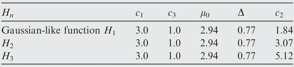
Table 6 Parameter selection for different Hn functions.

Fig. 20 Processed results of Hn curves.
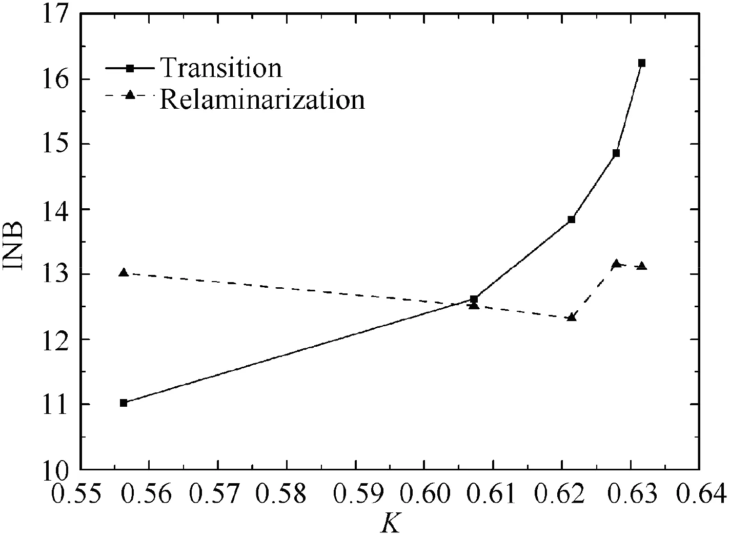
Fig. 21 The INB value varies with slope K of function.
As previously known, the cumulative function slope K of the Hnfunction increases as n increases.Therefore,the increase of n can increase the INB value of the left boundary of the magnified area, however it has a nonlinear effect on the right boundary. The Hnfunction should be the step function when it obtains the maximum INB value targeting the left boundary of the magnified area.
Although the increase of n increases the INB value of the left boundary of the magnified area,it imposes higher requirements on the accuracy of the boundary.In actual situations,it is often impossible to obtain a precise magnified area. In this case, we suggest that the n value should not be too large,and n can be taken as n=1,that is,the Gaussian-like function can be selected.
Further, the VSWT will degenerate into the SWT when n=0. When n=0, the value of Hnis H0=c1+c3. In such case, the window function does not change as RMS/RMS0changes. It can be seen that the SWT developed in paper13is only a special case of the VSWT developed in this paper. The VSWT has a wider range of applications.
4. Results
Experimental data of the S809 airfoil and the NACA0012 airfoil is processed using the VSWT discussed previously.The Hnfunction is selected as the H1function, which is the Gaussianlike function.
4.1. Results of S809 airfoil
In this section, the experimental data of the S809 airfoil are processed. And the model chord length was c=500 mm, the Reynolds number was Re=0.75×10⁶and the reduced frequency were k=0.1571 and k=0.2356.
(1) Case of k=0.1571
In the case of k=0.1571, the magnification of transition/relaminarization at each point of the airfoil can be referred to Fig. 12. The suggested value of the parameters for global calculation strategy can be obtained according to Fig. 12 as shown in Table 7. In the single point calculation strategy, c2is taken as c2=8.0 to ensure a sufficient large INB value.
The calculation results of different methods in the case of reduced frequency k=0.1571 are shown in Fig. 22. It can be seen that the feature obtained by the VSWT developed in this paper is more obvious than that obtained by the SWT at feature positions.
In order to quantitatively evaluate these three methods,the INB values and the Δα at the feature positions are calculated as shown in Fig. 23. Same as Fig. 16, the results of the SWT are represented using black color; the results of the G VSWT are represented using red color and the results of the SP VSWT are represented using blue color. It can be seen that the INB values calculated by the VSWT developed in this paper are obviously improved and the Δα are significantly reduced compared with the results obtained by the SWT in the case of k=0.1571.
(2) Case of k=0.2356
In the case of k=0.2356, the magnification of transition/relaminarization at each point of the airfoil can also be referred to Fig. 12. The suggested value of the parameters for global calculation strategy can be obtained according to Fig. 12 as shown in Table 8. In the single point calculationstrategy, c2is taken as c2=8.0 to ensure a sufficient large INB value.
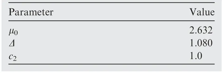
Table 7 Suggested value of parameters for global strategy in case of k=0.1571.
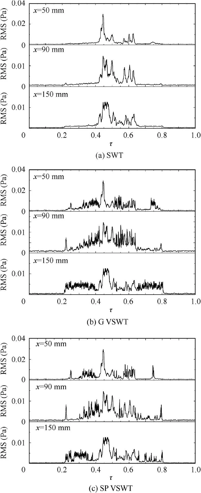
Fig. 22 Results of different calculation strategies in case of k=0.1571.
The calculation results of different methods in the case of reduced frequency k=0.2356 are shown in Fig. 24. It can be seen that the feature obtained by the VSWT developed in this paper is more obvious than that obtained by the SWT at feature positions in the case of k=0.2356.
The INB values and the Δα of different calculation strategies in the case of k=0.2356 at feature positions are shown in Fig. 25. It can be seen that the INB value calculated by the VSWT developed in this paper is still obviously improved and the Δα are still significantly reduced compared with the results obtained by the SWT in the case of k=0.2356.
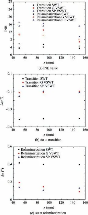
Fig. 23 INB value and the error of angle of attack Δα of different calculation strategies in the case of k=0.1571.
4.2. Results of NACA0012 airfoil
The experimental data of NACA0012 airfoil is also processed in this paper to further validate the developed VSWT.
The experimental model has a chord length of c=700 mm.The experimental Reynolds number was Re=1.0×10⁶. The average angle of attack of the model pitching motion was α0=10°and the amplitude was A=10°. The oscillation frequency was f=1.0 Hz, so the reduced frequency was k=2πfc/U∞=0.192.
The suggested value of the parameters for global calculation strategy are shown in Table 9.In the single point calculation strategy,c2is taken as c2=8.0 to ensure a sufficient large INB value. The remaining parameters are consistent with the parameters used in previous S809 airfoil.
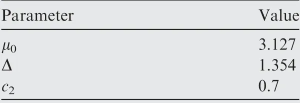
Table 8 Suggested value of parameters for global strategy in case of k=0.2356.
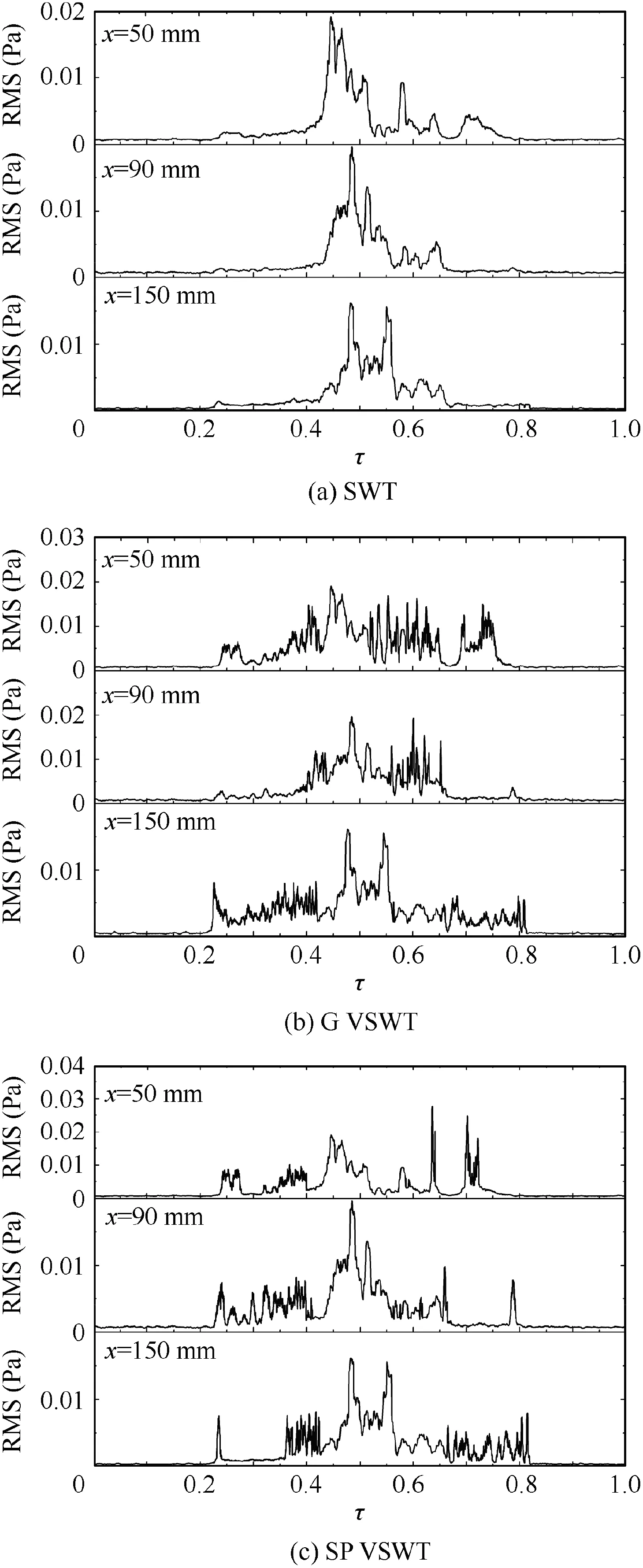
Fig. 24 Results of different calculation strategies in case of k=0.2356.
The calculation results of different methods in the case of reduced frequency k=0.192 of the NACA0012 airfoil are shown in Fig. 26. It can be seen that the feature obtained by the VSWT developed in this paper is still more obvious than that obtained by the SWT at feature positions for the NACA0012 airfoil.
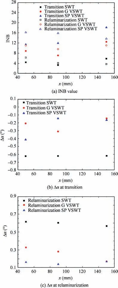
Fig. 25 INB value and error of angle of attack Δα of different calculation strategies in case of k=0.2356.
The INB values and the Δα of different calculation strategies at feature positions are shown in Fig. 27. It can be seen that the INB value calculated by the VSWT developed in this paper is still obviously improved and the Δα are still significantly reduced compared with the results obtained by the SWT for the NACA0012 airfoil.
We propose two computing strategies, global strategy and single point strategy, for the VSWT. The single point strategy can obtain a higher INB value than the global strategy,but the RMS magnification at the feature position need to be known in advance which brings difficulties to practical applications.The global strategy can improve this situation.The RMS magnification at the feature position does not need to be known in advance in the global strategy. And a satisfactory results can be obtained by simply giving a magnified area.
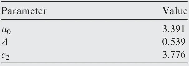
Table 9 Suggested value of parameters for global strategy of NACA0012 airfoil.

Fig. 26 Results of different calculation strategies for NACA0012 in case of k=0.192.
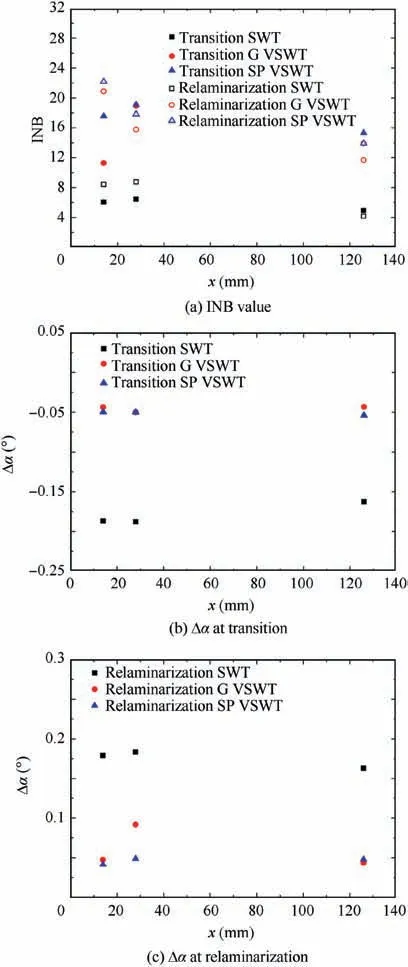
Fig. 27 INB value and error of angle of attack Δα of different calculation strategies for NACA0012.
5. Conclusions
A more practical Variable Slip Window Technology (VSWT)is developed in this paper using the fluctuating pressure data of the S809 airfoil based on the Ref.13.We propose two computing strategies: global strategy and single point strategy for the VSWT. The core of this technology is the selection of the window function h and the parameters setting in h function.Both computing strategies have their own advantages and disadvantages. The single point calculation strategy can achieve a higher INB value, but the RMS magnification at the feature position needs to be known in advance. The INB value obtained by the global strategy is slightly smaller than the calculation results of the single point strategy.In addition,it is not necessary to known the RMS magnification at the feature position in advance. So the global strategy has better robustness.The errors of angle of attack Δα of both computing strategies are smaller compared with that of SWT.Considering the actual situation, we suggest using the global strategy to process the airfoil dynamic data.
The characteristics of h function have a significant influence on the VSWT. The suitable functions are Hnfunctions constructed in this paper and step function. In particular, the VSWT will degenerate into the SWT when using H0function(n=0). For the left boundary of the magnified area, the step function can obtain the largest INB value,but the robustness is not good.The H1function(Gaussian-like function,n=1)can show higher robustness while guaranteeing a large INB value.In practical applications,we propose to choose the H1function(Gaussian-like function) as the h function.
In addition,the experimental data of the NACA0012 airfoil is also used to further validate the developed technology. The results show that the VSWT developed in this paper can still double the INB value and the Δα are still significantly reduced at the transition/relaminarization position.
The VSWT developed in this paper is a generalization of the SWT and possesses a wider range of applications. The VSWT can highlight the transition/relaminarization characteristics,which can facilitate automatic recognition by the computer.
Acknowledgements
Thanks all the staff in NF-3 Lab very much for their hard work and help in the wind tunnel experiment. At the same time, we would like to thank the Youth Science Foundation(No. 20181111502212) for their support.
杂志排行

CHINESE JOURNAL OF AERONAUTICS的其它文章
- Reliability and reliability sensitivity analysis of structure by combining adaptive linked importance sampling and Kriging reliability method
- Aeroelastic dynamic response of elastic aircraft with consideration of two-dimensional discrete gust excitation
- Thermal damage analysis of aircraft composite laminate suffered from lightning swept stroke and arc propagation
- An aerospace bracket designed by thermo-elastic topology optimization and manufactured by additive manufacturing
- Applications of structural efficiency assessment method on structural-mechanical characteristics integrated design in aero-engines
- An energy-based coupling degradation propagation model and its application to aviation actuationsystem