Model-driven degradation modeling approaches:Investigation and review
2020-06-11RuiKANGWenjunGONGYunxiaCHEN
Rui KANG, Wenjun GONG, Yunxia CHEN
School of Reliability and Systems Engineering, Beihang University, Beijing 100083, China
KEYWORDS Degradation law;Degradation process;Meta-models;Multi-mechanism;Multi-performance
Abstract The second law of thermodynamics implies that any animate and inanimate systems degrade and inevitably stops functioning. It is irreversible over time that can be labeled as ‘‘the degradation arrow of time”.From perspective of products’reliability design,it is essential to build appropriate models of describing the degradation arrow of time.The current modeling approaches mainly include the model-driven(having assumed forms based on cognitive experience of mankind)and data-driven (using data learning techniques without form hypothesis) approaches. In this paper, we just investigate and review the model-driven degradation approaches, hoping to provide suggestions of the model construction or selection for scholars or engineers. First, for the single mechanism, degradation law models and stochastic process models are classified as separately depicting the tendency and fluctuation of degradation.For the degradation law model,we propose the concept of meta-models as original types for various personal models.For the stochastic process model,two main types including the non-monotonic and monotonical types are presented.Then,four multi-mechanism degradation types are discussed, that are competitive degradation, multi-stage degradation, coexistence of degradation and impact, and coexistence of degradation and failure.Besides, for the multi-performance degradation, independent and coupling models are introduced.The forms,connotations,applicability and insufficiency of these models are described with a series of examples from the literature and our own experiences. The final explicit suggestions about the potential future work are provided for the development of new degradation models.
1. Introduction
1.1. Motivation
Today’s industry and manufactures has a growing strong demand for developing higher-reliability, longer-life products in record time.1Generally,these modern products can operate without failure for years, decades or even longer. It brings a tremendous challenge of estimating their failure-time distribution.2To assess the life or reliability levels of such products, methods using degradation data develops in a short time.3-5
The fact is that degradation becomes a common feature of things in our world; it reflects the principle of the second law of thermodynamics, which is ‘‘the entropy of an isolated system (disorder) increases with time”. Compared to the lifetime data, degradation data contains more information about product’s performance changes. To some extents,the degradation refers to some processes like physical loss or chemical reactions may cause the failure partially.6,7Therefore, a ‘‘degradation mechanism” can be a physical,chemical, or other process that causes a gradual change in a product’s characteristic quantities. Sometimes, the multimechanism degradation would happen due to the structural or functional interaction, which refers to the phenomenon that several product’s characteristics undergo gradual physical and chemical processes with coupling relationship. It shows obvious differences compared with other typical single physical mechanism. These coupling effects have been confirmed in many areas like electronics, machinery, electrical fields.8-10Sometimes, degradation is reflected by performance changes. The performance is representing outside characteristic of products caused by inner coupling with environment effects.11Such as mechanical properties, electrical properties, thermal properties, optical properties, magnetic properties. In general, it can be quantitatively described by the corresponding physical and chemical processes, reflected by performance parameters. When the product is operating under external working stress and environmental conditions, performance parameters will degenerate. When the performance parameters degrade to a certain extent that is not enough to meet the needs of normal working, the failure occurs. For the product with complicated structure and diverse functions, degradation processes of multiple performance parameters appear simultaneously, presenting the multi-performance degradation characteristics. Thus, studies on the degradation modelling include single mechanism, multi-mechanism, multiperformance degradations.
From 1980s, the degradation phenomenon has attracted wide attention of scholars.12,13Various degradation models based on different mathematical principles and assumptions emerge. Some of them are demonstrated by practical engineering about their suitability and accuracy. They are mainly classified into two classes: (A) model-driven; (B) data-driven.The concept of model-driven and data-driven approaches originally come from the software system modelling. Their distinguish is listed as follows: The data-driven approach means that progress in an activity is compelled by data,rather than by intuition or by personal experience. While the model-driven approaches provide a set of guidelines for the structure and forms of models. Throughout this paper,we just focus on model-driven approaches for the degradation modelling. The purpose of this paper is to outline some of the basic ideas behind model-driven degradation methods for providing some reasonable thoughts when building a new degradation model. So, in our concluding remarks, explicit suggestions are given from the literature and our own experiences.
1.2. Model-driven approaches
For products, the deteriorating process is unavoidable, sometimes there maybe just one or more parameters that we can find to describe the degradation path. For one parameter,the existing studies on the degradation modelling based on the model-driven approaches mainly include single mechanism, multi-mechanism degradation. For two and more parameters, we call it multi-performance degradations. The classification scheme of these models is visually presented in Fig. 1. Before discussing the detailed description of modeldriven approaches, the concept of ‘‘model-driven” from our perspectives means that some assumptions for structures of models are provided by the cognitive knowledge of mankind.
The typical single-mechanism degradation can be classified into ‘‘Degradation Law Modelling” (DLM) and ‘‘Stochastic Process Modelling” (SPM). A DLM model is to describe the development tendency of the degradation level. A deterministic mathematic form is commonly needed to describe the tendency. By analyzing the mathematical forms of different degradation models.We can sum up the following conclusion:Many degradation models applied in different areas with the similar function forms can trace back to an original degradation model. We called these original degradation models as meta-models, having the similar concept existed in computational science. These meta-models have deterministic physical meanings that can reflect basic laws of degradation phenomena. Some rules from them can be utilized to learn how to establish an appropriate model for depicting the similar degradation tendency in a short time. However, just knowing the degradation tendency is not enough; their presented degradation process is a single ideal and smooth degradation line. It requests the complete consistency of products and the working& environmental conditions. In practice, individual difference and various conditions make products cannot fail at the same time.Besides,the degradation process of each product shows a rough and non-smooth curve. Therefore, stochastic process models are developed to make up for the shortage of these deterministic degradation models.
A SPM model is a kind of degradation model that can both reflect the trend and fluctuation of degradation. The fluctuation of degradation is commonly described by uncertainties;they are mainly from the subjective and environmental conditions, which includes the stochastic or inherent uncertainty that cannot be eliminated,such as the difference between samples, physical measurement error, and the cognitive uncertainty due to the lack of information. The existing degradation modelling method only consider the influence of stochastic uncertainty, which is described by stochastic processes like random coefficient regression equation, Poisson process, Wiener process, Inverse Gaussian process and some other models that we can find in literatures.
In addition, multi-mechanism degradation phenomena are common in many areas. With the effect of multi-mechanism,the degradation path is not usual as the general type that is monotonic and continuously uninterrupted. The key point about how to describe the multi-mechanism is to understand the modelling principle of the single-mechanism degradation and coupling relationship between these mechanisms.The coupling relationship between these degradation mechanisms draw many scholars’attention.In this paper,four typical cases are presented to reflect the multi-mechanism degradation characteristics. They are competitive degradation, multi-stage degradation, coexistence of degradation and shock, and coexistence of degradation and failure. These four cases can only cover the situation that coupling mechanism can be described clearly.However,in most cases,it is difficult to explain the socalled coupling relationship in detail,how to solve the problem of life prediction under the coupling condition is the key point in the future research.

Fig. 1 Scheme of model-driven degradation modeling approaches: investigation and review.
Moreover,the above description of the modeling method is mainly for the degradation process with single parameter that could be related single-unit systems(or systems considered as a whole). With the development of structure complexity and functional variety, products under concerned circumstances usually undergo the multi-parameter degradation processes,which reminds us to elaborate on the degradation modeling of multi-performance parameters for multi-unit systems. In the multi-performance degradation area,various types of independence or dependence structure incorporated in multivariate models are the important parts for evaluating the system reliability. The related research work can be classified into two patterns: 1) independent multi-performance degradation; 2)coupling multi-performance degradation. Some methods for each pattern are discussed in this paper to provide various understanding of multivariate degradation modelling.
In final, we further introduce the applications of degradation modeling that include the Remaining Useful Life (RUL)estimation and degradation-based maintenance policy. RUL is an essential part in prognostics and health management.Model-based RUL methods consider the data partially indicating the underlying state of the system and assumed that the available degradation data were stochastically related to the underlying health state.Besides,Degradation-Based Maintenance (DBM) policy has also drawn attentions from many scholars to reduce the potential failure and accidents. It can be concluded, according to their efficiency, into three types:perfect maintenance, minimal maintenance and imperfect maintenance.In here,the imperfect maintenance is further discussed by analyzing its positive and negative effect.
1.3. Overview
The remainder is organized as follows. Section 2 describes the basic physical and practical ideas behind the single mechanism degradation model. The concept of the multi-mechanism degradation modelling and four difference cases are introduced in Section 3.Section 4 presents the life prediction methods of products with multi-parameter degradation. Section 5 makes a conclusion and prospects some work of future research.
2. Typical single-mechanism degradation
2.1. Degradation law model
Basically, the degradation law model is a mathematical formula is constructed that represents the intrinsic physical or chemical degradation process.It can directly reflect the impact of design parameters on the degradation process like structure,material, processing technology etc. Depending on the type of output variable, the model applies to different product types that can be divided into electronic and non-electronic types.It mainly establishes the functional relationship between degradation time or degradation quantity and the degradation cause(such as the environmental factors).Analyzing the mathematical form of these models, we can conclude that many models having different types can be traced back to the same original physics-based model. These original models can be regarded as basic models of personal models. They can also be named as meta-models, having the similar concept existed in computational science.14From literatures, we generalize the commonly used meta-models (includes Arrhenius, Archard, Paris equations, etc.) from background, forms, modifications,development,and applications.It needs to be noted that the mentioned meta-models in here are the classical model forms verified through decades. So, a meta-model can explain the common essence of degradation mechanism, implying the difficulty to propose a new meta-model.

In 1889,Arrhenius15proposed an empirical physical model- ‘‘the Arrhenius Model”, based on the observation of experimental data when studying the thermal chemistry reactions.It concludes that the reaction rate k is inversely proportional to the exponent of the activation energy Eaand inversely proportional to the exponent of the inverse of the absolute temperature Te, that is where kBis the Boltzmann constant, C0is the proportional constant.The Arrhenius relationship has been widely accepted by scholars and engineers, which is utilized in many applications.16However, the Arrhenius equation does not apply to all temperature acceleration problems and will be adequate over only a limited temperature range. Nelson17comments that ‘‘... in certain applications (e.g., motor insulation), if the Arrhenius relationship...does not fit the data, the data are suspect rather than the relationship”. In 1935, Henry18applied quantum mechanics and statistical mechanics into the Arrhenius Model, and developed the theory of absolute rate and the theory of effective liquid structure. The main difference between the Eyring model and the Arrhenius model is that there is a power law term including the temperature stress before the exponential term. In 1972, Weston and Schwarz19made a detailed description of Eyring model from the point view of chemical kinetics. In addition, Mcpherson20proposed a generalized Eyring model cover other stress types such as voltage, humidity.

where h is the Planck constant,Siis the ith stress type,fiis the function of Si. C0, ci, and diare constants. In 2006, Escobar and Meeker2used the Eyring model to describe the failure mechanism of solid-state electronic devices. They pointed out that if the temperature satisfied the exponential relationship,Eyring model is more suitable to get an accurate result onto extrapolation, compared with the Arrhenius model.
In 1953,Archard21attempted to develop a theoretical basis to explain the wear of materials as
where K is the wear coefficient,P is the contact force,σsis the yield limit of the worn material. Eq. (3) has been one of the most acceptable wear equations. However, the value of K in the model can only be determined experimentally or empirically, leading to inaccurate prediction results; and it cannot describe the complex wear mechanism.20In last decades,there have been more than 300 related formulas being proposed,but even the best formula has many limitations. Meng and Ludema22pointed out that many contact calculation formulas simply consider the wear coefficient as a constant, without considering time-related effect from the wear process, which greatly restricts their application areas.
In 1961,Paris et al.23used the fracture mechanics theory to derive the crack propagation law and put forward the famous Paris’s Law. The basic formula reads

where a is the crack length and da/dN is the crack growth rate,which denotes the crack growth for a load cycle.On the righthand side,C and m are constants that depend on the material,environment and stress ratio,and ΔK is the range of the stress intensity factor during the fatigue cycle.As one of the common equations in fatigue, Paris’ Law is suitable for describing the stage II crack growth with cycles.Other scholars then modified it in many ways to make better allowance for applications.24In 1993,Lu and Meeker25used the Paris’Law as the degradation track function for a set of crack fatigue data.In 1998,Meeker et al.26studied the edge crack growth of metal plates using the Paris’ Law. In 2005, Zhao et al.27explained the degradation data of helicopter rotating devices based on the Paris’ Law.
These above meta-models are the basis of numerous personal models for products with their own parameters.Besides,from the perspective of mathematics, three basic forms can be concluded7: power law form, exponential form, and logarithmic equation. It seems that a possible mapping relationship database exists between mathematic forms and degradation mechanisms caused by various stresses, like the exponential relation of temperature, or the power law form of mechanical stresses. So, some practical ideas from these meta-models could be proposed for building an available degradation model in a short time. In 1983, Takeda and Suzuki28used the power law form to study the degradation process of the volt threshold of electric device. It is widely applied in electric stress-related failures like voltage,current,power,etc.In 1994,Chan et al.29described the degradation character of film resistor with the power law function. Wang30studied the degradation data of electronic components and established the degenerate trajectory function based on the power law form under accelerated stress.An improved least-squares estimation of the parameters was given to evaluate the average life of the product. In 2005,Gabraeel et al.31used the exponential form to describe the degradation signals of the gears and used the Bayesian method to combine the historical data with the current detection data to predict the residual useful life of a single gear in real time.As a special case of power law form. The linear form is commonly used in engineering. In 2014, Yang et al.32described the electric meter’s degradation under accelerated stress with the linear model. In 2014, Baussaron et al.33mentioned that a weighted linear model to describe different simulation data and gave fairly good results in all cases that can be a good compromise.In addition,the general logarithmic form is commonly used to analyze the compression spring stress relaxation.34,35
2.2. Stochastic process model
In the early stage, scholars’ intention is just to obtain the degradation trend by the degradation law model,just showing a single ideal and smooth degradation line. However, individual difference and various conditions make products degrading with fluctuation. So, the degradation shows a rough and nonsmooth curve. Therefore, degradation process models are developed to make up for the shortage of these deterministic degradation models. Naturally, using the stochastic process for the modelling would be the first thought from many scholars. The stochastic process characterizes the temporal uncertainty of the degradation process and the random influence from the operating environment, which can well make up for the shortage of the deterministic degradation. Since Mercer and Smith36may firstly describe deterioration by a stochastic process in 1959, it has been through more than sixty years for development in the stochastic degradation process. The current stochastic processes applied into the degradation modelling mainly include the random coefficient regression equation, the Poisson process, Wiener process, Gamma process,and Inverse Gaussian process.When talking about these models,we are trying to make a classification of them.After studying their mathematic feature, we try to classify them into two types: the monotonic degradation and the non-monotonicdegradation processes. The classification of common stochastic process model has been presented in Table 1.37-65

Table 1 Classification of common stochastic process models.
2.2.1. Non-monotonic stochastic processes
Non-monotonic stochastic processes refer to processes that the degradation is reversable over time like random coefficient regression model and Wiener process, Poisson process,etc. Random coefficient regression model assumes that the degradation process consists of the theoretical variation of deterioration process and the random error in each sample path. As the origin of this model, a simplified form was firstly proposed by Sheiner and Beal in 198037in the study of pharmacokinetics. Then,Seber and Wild (1989)38further provided theory of this model in areas like economics and social science, etc. Lu and Meeker (1989),39Nelson (1990)17reviewed references on random efficient models and introduced the applications in the degradation area. Based on the generalized form from Lu & Meeker25and Wang’s30hypothesis, uncertainties from the error term,40,41and degradation data42are further studied. The general form is presented as

where η is the theoretical degradation volume, φ is the fixed effect item, Θ is the random effect item. ε is the error term.The degradation path modeling method can describe the performance degradation process of products very well, and it has a wide range of applications in ADT data processing.66The models can describe stochastic uncertainties, including measurement uncertainty and sample difference. However,the product’s intrinsic degradation can be influenced by the material and environment,and the instantaneous performance degradation exists random uncertainty as well. These above factors are not included in the degradation path model.It limits the application of degradation path model to a certain extent.
The Wiener process model including the drift and the diffusion parts is suitable for those processes where the degradation trend varies linearly with time and has Brownian motion noise.67Basic theoretical properties of a Wiener process may be first found in Cox and Miller(1965).68It is often called standard Brownian motion process due to its historical connection with the physical process known as Brownian motion originally observed by Robert Brown in 1827.69In 1921, Wiener70made an accurate mathematic description for the Brownian motion, and further put forward the estimate and integral types of Brownian motion space. Sherif and Smith43pointed out the connection between degradation and Wiener process.44In 1993, Doksum and Hoyland firstly applied the wiener process into the accelerated life test.45Then, the development of Wiener process in the degradation area can be classified into three terms: (A) measurement errors; (B) stress factors; (C)random effects. Ye71and Si72et al. made a comprehensive review work in these terms.
The Poisson process model is mainly used to describe the degradation process of a product that is subject to multiple‘‘bumps” before it fails.53From a historical point of view,the Poisson process was invented by Filip Lundberg62firstly with in consideration of temporal and spatial development of Poisson distribution.The Poisson process is commonly applied to the accumulated shock models. In 1959, Mercer and Smith first36modeled the wear as a compound Poisson process.Then,modified models with different assumptions are established in literatures.53-55,73-74Koroliuk et al.75reviewed the related work and made a good interpretation of these models.
2.2.2. Monotonical stochastic process
In contrary, monotonically increasing processes that assume the degradation is irreversible which can describe most actual situations like gamma process, Inverse Gaussian (IG) process,etc. The gamma process is a stochastic process with independent, non-negative increments having a gamma distribution with an identical scale parameter.76It is a natural model for the degradation processes with a sequence of tiny positive increments.77Gamma process can be regarded as a limit of the compound Poisson process.57When the strength of Poisson process tends to be infinite, and the jumping interval to a certain extent gets close to zero,the compound Poisson process has become the Gamma process. It can be well applied into the degradation caused by external shocks with random and small magnitude. In 1975, the gamma process was first applied by Abdel-Hameed56as a model for deterioration occurring random in time.van Noortwijk76reviewed the development of gamma process in the last three decades, such as creep,58fatigue,76corrosion,59maintenance.60,61It provides an excellent reference for the study of gamma process.
The IG process is another alternative statistical process with monotone increments, which is suitable in degradation modelling.Inversely related to the Wiener process,the IG process is defined as the increment satisfying an IG distribution.73It was proposed by Wasan78in 1968, has not been extensively applied into degradation area owing to unobvious physical meaning.62,79To bridge the gap,Ye and Chen63further studied the physical meanings of IG process. They found that the IG process is also a limit of compound Poisson processes like the Gamma process. The lexibility is outstanding in terms of modelling stress factors and random effect into the basic model.64,78Nevertheless,the IG process still needs more attention in the degradation area.Properties of the process and further explanation should be studied to provide theoretical support for the application in the degradation modelling.
2.2.3. Others
In 1985, Bognadoff and Kozin80proposed the Markov chain model to describe the degradation process. Markov chains are an important class of probability models. The model assumes that the damage caused by each stress cycle is independent of the current accumulated damage and can be described by a homogeneous Markov chain. In practice, it is only applied into the preventive maintenance modelling.65The reason might exist that the assumptions are too ‘‘harsh”,which makes it hardly correspond to the actual situations very well. The Markov chain model considers a discrete degradation space whereas Wiener, Gamma or Inverse Gaussian processes are with continuous degradation. Hence real situations adapted to Markov chains are very specific, but it can be a way to obtain a simplify modeling framework.
Generally, a good stochastic process model should satisfy several requirements50: (A) clear physical explanations; (B)concise forms for easily understand;(C)good properties, such as easily incorporating prior information and flexible stress factors and random effects.The most common used stochastic process models can meet all these requirements that are, the Wiener process, Gamma process and IG process. In actual,we admit that a stochastic process is to model the unexplained randomness from unobserved environmental factors. Once a new physical finding or theory can explain the nature of the randomness, more accurate and mature model combining new thoughts should be considered for the degradation process.
3. Multi-mechanism degradation
The degradation mechanism of typical single mechanism has been extensively applied to many products,proving its validity and accuracy. However, in practice, due to the complexity of the product itself and the uncertainty of external factors, the degradation process is often accompanied by a variety of failure mechanisms.In addition,the failure mechanisms often present a coupling relationship, which affect the degradation characteristics of the product. It is obviously different from the typical single mechanism degradation characteristic.Multi-mechanism degeneration has been widely recognized in the field of electronics and mechanics.81The typical multimechanism coupling phenomena as Table 282-115presented are classified into: (A) competitive degradation, (B) multistage degradation, (C) coexistence of degradation and shock,and (D) coexistence of degradation and failure.
3.1. Competitive degradation
With respect to the competitive degradation model, different scholars may have different understandings.A typical competitive degradation model is used to identify the models based on the‘‘take short” principle.Austen and McIntyre82argues that mechanical fatigue and stress corrosion do not appear to be superimposed in some cases,but rather a process that is faster to represent the crack growth process, that is the competitive model. In 2009, Bocchetti et al.83reported two major failure mechanisms, wear degradation and thermal cracking when analyzing the reliability of marine oil cylinder liners. When one of these two mechanisms reach the failure threshold,a failure occurs.Slee et al.84considered the failure of printed circuit boards, pointing out that different failure mechanisms could lead to failure of the circuit board, including fatigue of solder joints caused by cyclic thermal loads, fatigue due to platedhole contamination,and electron thermal migration,and these kinds of failure mechanisms exist competition.
In 2010, McPherson7pointed out that one mechanism might increase the critical parameters of the material/period while the other causes the key parameter to decrease. These two mechanisms compete, resulting in that the performance parameter reaches to a maximum or minimum value during the degradation.For instance,it is often necessary to establish good connections by diffusion of the two materials near each other at different temperatures. Initially, the inter-diffusion between the two materials increases the interfacial link strength, however as the inter-diffusion continues, the formation of the Kirkendahl hole near the interface causes the bond strength to begin to decrease. The degradation process can be described as

where the first part on the right side represents the increasing mechanism of S; the second part on the right side decreasethe value of S; and A0, B0, m1, m2are estimated coefficients.This model is the general mathematical form as for this kind of competitive degradation mechanism, which is the multiplication of two deterministic degeneracy laws (one representing the growth mechanism and the other representing the reduction mechanism).However,this model cannot effectively characterize the actual degradation process with uncertainties.Second, in the degradation model, the relationship between the two degradation mechanisms is certain and time dependent. In addition, the degradation may show that the actual product degradation and stress conditions have a great relationship that the coupling between the two degradation mechanisms are changing.In practice,the environmental load often changes; so, the time-varying load characteristics of product degradation should be included in the model.

Table 2 Classification of multi-mechanism degradation models.
In 2007, Moens et al.85proposed a physical model for LDMOS transistors to calculate the degradation behavior under alternating current conditions from hot carrier data under direct current conditions. They found that with the injection of hot holes, a new interface is formed that has the opposite effect on the degradation of the on-resistance and occupies a dominant low level at some stage,so that the degradation path exhibits a tipping point. Sun et al.86pointed out that different mechanisms under different stress conditions,in the degradation process of the resistance would occupy different positions.Under the conditions of low gate voltage and high leakage voltage, two kinds of competing degradation mechanisms are mainly presented. The hot hole injection in the beak region and the interface state in the channel region cause the on-resistance of the device to vary with stress and time increasing which was first decreased and then increased.Amat et al.87studied the degradation behavior of channel hot carriers in N-MOS transistors fabricated from high dielectric constant materials. They pointed out that their degradation behavior can be divided into two parts. At different temperature levels, different degradation mechanisms will occupy the dominant position, which has a great impact on the degradation characteristics and product lifetime.In the literature, the degeneration of MOS transistors is mostly explained by experimental phenomena and data from the physical point of view, and no general mathematical model has been established. For different types of products, it is difficult to build a new physical model directly through the degradation characteristics.
3.2. Multi-stage degradation
In practice,multi-stage degradation may occur due to the complexity of the composition of the product structure and the diversity of the environmental stresses. A typical multi-stage degradation is a degradation delay phenomenon. Sometimes materials/devices will be remarkably stable for a period t0and then show relatively rapid degradation with time.The first stage occurs when the product begins to work for a period without degradation. After that, the product begins to degradation until the failure. For example, a tire with a stable tire pressure can be stably operated for a period after the tire has been nailed; the resistance of the metal conductor is stable before the inside is formed; the fuel efficiency of the engine is also stable before the nozzle is blocked. In 1976, Christer first proposed the delay-time concept to justify the necessity of inspection activities for plant preventive maintenance.86The basic model proposed by McPherson equals7
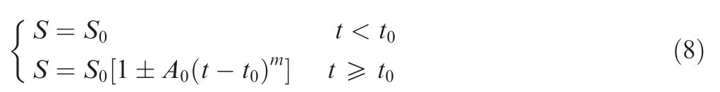
where, S is the important material/device parameter, S0is initial value of the parameter, and t0is the degradation delay time. the+sign is used when S increases with time whereas the - sign is used when S decreases with time. This model just makes an explicit and deterministic model for the degradation delay behavior without any uncertainties. The measurement error or environmental factors still affect the delay degradation process. Thus, in 1995, Nelson116proposed a linear regression model with the normal distribution for the delay growth of blisters on metal sheets and the two-phase dendrite size growth. In this model, the sample dispersion is considered by using the initiation time and failure time distributions. Then,Nelson117also mentioned that a more complicated model with measurement error would appear in the further study.In 2013,Guo et al.118also proposed a two-step strategy for modeling degradation with an initiation time. The exponential form is proposed with an initiation time point t0for describing the two-stage degradation. For identifying the initiation time point, two methods that can be utilized to obtain degradation data in modeling.If there are enough readings after the degradation starts, straight observation would be used. If there are not enough readings, or the variability between readings is high, statistical process control is recommended. All these above models just make a good starting for the delay-time degradation modeling.The deficiencies still exist that it cannot reflect the environmental factors and the instinct uncertainty of degradation process.
Besides, during the degradation process of some highreliable products, the inner structure and material changes with time increasing.It leads to different characteristics of system degradation behavior. For example, Spotnitz119pointed out that the capacity degradation of lithium batteries consists of four stages with different degradation rates. The root cause is related to the lithium ion loss caused by different chemical reactions. In 2008, Ng88considered that a class of product’s degradation processes consisted of different stages. When the potential degradation process of a stage changed,the degradation rate at that time would increase or decrease.He proposed a stochastic process like Wiener process or compound Poisson process using independent increments with a potential turning point for stochastic change to establish a degradation model for the multi-stage degradation problem.In 2012,Feng et al.89investigated the capacitance increasing of the high-voltagepulse capacitor, which is used to store and discharge electrical energy rapidly. The experimental results indicate that capacitor undergoes three-stage degradation process. That is, the capacitance increases slowly or fluctuates in the initial storage stage. Then it increases sharply in the middle stage. After the two stages,the capacitor enters the third stage in which capacitance increases constantly. Authors chose a multi-phase Wiener process involving change points to model the degradation process with the experimental data. The proposed approach is useful for the performance characteristic, which could be extended to other long-storage products in many applications. In 2013, Chen and Tsui90analyzed the degradation signal of gear vibration using a two-stage variable-point model and used the Bayesian method to integrate the historical data and the real-time detection data to predict the residual useful life of the gear. The prediction results of the two-stage degradation model are more accurate than the model just considering a second-stage degradation process. In 2015, Bae et al.91also used this method to analyze the degradation trajectory of a plasma display. In 2017, Li et al.92investigated the performance degradation of the airborne fuel pump that shows nonlinear and multi-stage with stationary-accelerated-station ary degradation pattern. They creatively introduced the Smooth Transition Auto-Regression method to capture the dynamic degradation process, which lays better foundation for the Prognostics and Health Management(PHM)of the airborne fuel pump.
In summary,the multi-stage degradation pattern has been a common phenomenon in many areas. These products with high reliability usually work for a long lifetime. It brings a problem that how to build an appropriate model to describe these degradation characteristics. The early method using the data regression model is not available for products with complex structure. The reasons are concluded that they cannot reflect the environmental factors and the instinct uncertainty of degradation process. Another modeling direction for making up these deficiencies are to consider a multi-phase degradation quantity models that may consist of different stochastic processes.For instance,the Wiener process can be appropriate for the first stage,while the Gamma or other stochastic process might be better for the second or other stages,or vice versa.In addition, the situation should be studied that the multi-stage degradation involves random change points.That is,products in the same type may undergo different change points, and how to incorporate the stochasticity of change points into the degradation process model is a challenging issue. The remainder can be classified into the various data-driven methods. Such as probabilistic method like Bayesian, filtering,machine learning data fusion,or others.However,these methods need a large amount of data from different sources to support their validity.Therefore,the fusion of degradation models and data-driven methods would be worthy of development for the multi-stage degradation.
3.3. Coexistence of degradation and shock
In the actual product use,it is often accompanied by the occurrence of the shock.The model considering the degradation and stochastic shock is called the Degradation-Threshold-Shock(DTS) model. In 1985, Lemoine and Wenocur93might first propose the DTS model.The degradation process is characterized by a diffusion process,and the fatal shock is characterized by a Poisson process.When the degradation reaches the preset value or when a fatal impact occurs, the product failed. In 2002, Klutke and Yang94established a system availability model with assumptions that degradation rate is uniform,and shock obeys the Poisson process. In 2005, Li and Pham95considered the existence of a variety of degradation processes and a shock process in the system itself. However, the above-mentioned literatures are based on the hypothesis of independence between the degradation and the shock. However, in practice, their coupling relationship with each other often exists that should be investigated. Current models describing their correlation can be divided into the shockassociated degradation model and the degradation-associated shock model.
The shock-associated degradation model assumed that the impact at each arrival would have an impact on the degradation process as

where Y(t)is accumulated by the function f(·)between natural degradation X(t) and additional damage S(t) caused by the shock. Shocks arriving at time tiis denoted as Wifor i=1,2,...,∞.The function has different forms that depends on different assumptions. In 2010, Peng et al.96assumed that each shock causes a sudden increase in the degradation rate and derived a probabilistic model to assess system reliability. In 2011, Wang and Pham97made predictive maintenance decisions based on this assumption.Keedy and Feng98applied this model to medical scaffolds,where the degradation process was derived from the failure physical equation. Jiang et al. considered the impact of the sudden increase in the phenomenon of degradation, but also considered the impact of hard failure threshold itself. They believed that after a series of shocks without failure, the hard failure threshold of the product would be reduced.In addition,in 2014,Rafiee et al.99assumed that the degradation rate would change with the arrival of different impacts. Wang et al.100considered that two different effects of the shock on the degradation process, including a sudden increase of the failure rate after a shock and a direct random change of the degradation level after the occurrence of a shock. In 2017, Zhang et al.101utilized the probability box to analyze the reliability of the system subject to the multiple dependent failure processes. Peng et al.96thought that previous models are too ideal to assume that precise model parameters are known beforehand.In practice,due to the limited resources,epistemic uncertainty would exist that can affect the reliability prediction. Therefore, an imprecise probabilitybased method like probability box innovatively are introduced into the shock-associated degradation models.
The degradation-associated shock model is another situation we need to consider.It assumes that the degradation process has an impact on the shock. One of general types can be concluded as102

where λ(t)is the intensity function of the random shocks,γais a dependence factor and X(·)is the degradation path,Θ is the random variable. In 1961, Mercer102proposed the original degradation-associated shock model of the form λ(t)+c·Z(t),where Z(t)is a degradation function describing the piecewise constant degradation process. Fan et al.103hypothesized in their paper that the magnitude of the shock increases with the degradation process.In 2004,Bagdonavicius et al.104assumed that the magnitude of the shock only depends on the degradation level.In 2011,Ye et al.105modeled the failure probability caused by the shock, which is increased as degradation process progresses. In 2017, Fan et al.106considered the degradation-shock dependence by establishing a linear function between the shock-induced failure intensity and the degradation level based on the Mercer’s assumption.102The developed model is applied to describe the dependent failure behavior of a sliding spool subject to wear and clamping stagnation. Then, Fan et al.107further developed a framework based on the Stochastic Hybrid Systems (SHS) to model and analyze systems that are subject to dependent degradation processes and random shocks. The developed framework is applied to model three failure patterns involving degradation-shock dependence from literatures.96,97,99The results demonstrate that the developed framework can yield an accurate estimation of reliability with less computational costs compared to traditional Monte Carlo-based methods.Besides, Yang et al.108,109considered the impact of discrete degradation on the shock from other perspectives such as the increases of the hazard rate108or the occurrence rate of shock.109It can effectively explain the failure behavior of systems like wind turbines, oil pipelines, electrical systems are exposed to random environmental stresses (e.g., harsh weathers, voltages, stress and temperature).
From these above literatures,we can easily find that the key issue to solve the dependent failure process involving degradation and shock is to propose a reasonable assumption on the relationship between the degradation characteristic and shock occurrence. The existing research about the shock impact on the degradation process can be classified into four terms: (A)shock occurrence increase the degradation rate; (B) the shock frequency can reduce the degradation threshold (a critical value being failed); (C) a shock can cause the sudden random change in the degradation level; (D) shocks make the direct increasing in the failure rate. Besides, the degradation process can also affect the shock happen mainly from these two aspects: (A) the magnitude of the shock only depends on the degradation level;(B)shock-induced failure intensity is a function of the degradation quantity.Regarding the interpretation of the coupling relationship between the degradation and shock. Some studies have been already out of the description of function and structure of actual systems.It will be very easy to become meaningless and purely into the mathematical logic game. To reflect the real situation of the degradation-shock dependence as much as possible, efforts of professional researchers are needed from other areas like physics or chemistry, to ensure the rationality and practicality of the relevant research.
3.4. Coexistence of degradation and failure
In practical engineering applications,there is a common situation that the degradation data and the failure data are mixed.Some scholars believe that the degradation-failure is belonged to the degradation-shock. It should be noted that the coexistence models of degradation-failure and degradation-shock have their overlap, because the shock can cause the product’s failure to some extents.However,there are some other reasons that can also cause the product’s failure.Sometimes,these reasons or mechanisms can be easily detected in the time-to-failure data because the failure mechanisms are slightly separated in time. Often, however, they are mixed (occurring during the same time intervals).In this case,a Kaplan-Meiers decoupling method is useful for separating the mechanisms as7

and
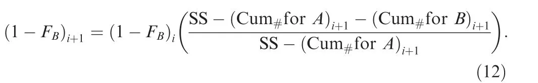
In the above equations, SS is the beginning sample size (at time zero)and Cum#represents the cumulative number of failures for each mechanism (A or B) at the indicated time interval. FAand FBseparately are percentages of cumulative failure numbers caused by mechanism A and B. Huang and Askin110pointed out that some electronic devices have two different failure modes. First, the degradation of light intensity,which is a degradation process, can be measured by the light intensity. The second one is the welding interface fracture,which is a catastrophic failure. They assumed that light intensity and the interface fracture time obey the Weibull distribution, and evaluated the product’s reliability based on the assumption of these two variables being independent. Based on this, Cha et al.111treated degraded samples as two distinct subpopulations for the reliability evaluation,including a weak subpopulation constituted by units with latent defects and a strong subpopulation. Later in 2016, they112also considered the correlation between parameters, and used the ternary normal distribution to describe their relationship.The existence of heterogeneous populations, a mixture of weak items and normal (or strong) items, is frequently encountered in most of manufactured products, Mixture models were also widely applied in the analysis of heterogeneous population.113Kim and Bai114used a mixture of two Weibull distributions to describe the failure data of an extrinsic and intrinsic failure modes.They assumed that a log-linear relation existed between the scale parameter and stress factor, and finally got the estimates of lifetime distribution. Normal degradation and defect failure modes have different accelerated relationships. Different responses to the same stress factors among different subpopulations need further investigation.115
These above four types reflect most multi-mechanism degradation phenomena.If we can clearly investigate the exact coupling process,deterministic mathematic forms can be written for these coupling relationships. Zeng et al.120made a discussion for coupling forms between mechanisms. They can be classified as competition, trigger, acceleration or inhibition,accumulation, etc. The corresponding research is based on the perspective of reductionism. It can make a good reference for other scholars. However, once the number of degradation mechanisms in a complicated system is considerable,the possible combinations of coupling relationships would increase rapidly to cause a combination explosion. Then, how to describe the system behavior becomes a challenging problem.This classic dilemma reminds us that we must reconsider another metrics or methods using the system theory to seek a breakthrough in the coupling effect characterization.
4. Degradation of multi-performance parameters
With the development of theory and engineering technology, product design, manufacturing processes, many products consisting of considerable components that may have several complex degradation mechanisms. It results in two or more performance parameters will gradually degrade over time. Sometimes these parameters may present a complex relationship including non-correlated, linear,non-linear or other situations. This above situation has already been observed in many actual engineering cases of different areas such as electronic equipment and complex structural products.121Indeed, many such bivariate and multivariate degradation concepts have already appeared in the literature for a longtime. Two pioneering pieces of work on multivariate degradation concepts were Harris (1970),122Thompson and Brindley (1972).123The related research work has been continued for a few decades.It can be classified into two patterns (see Table 3124-134):1) independent multi-performance degradation; 2) coupling multi-performance degradation.
4.1. Independent Multi-performance degradation
Multi-performance degradation modeling is based on the independence of the degradation parameters. Crowder135pointed out that independence hypothesis is valid if there is no direct or indirect association between the performance parameters. Crk136proposed a reliability evaluation method for multiple independent performance degradation processes.In 2005, Li and Pham124proposed a reliability model for the generalized polymorphic degradation system. It was assumed that the multi-performance degradation can be described by two independent discrete stochastic processes and a random shock. In 2008, Lu and Peng137gave a semi-parameter regression analysis to solve the modeling problem of multiperformance degradation processes. Therefore, the current work in the independent multi-performance degradation reminds us that if each performance degradation process can be modeled separately, we just assume that the system follows the series structure to model the system degradation process; and then the system reliability can be easily evaluated.
The multiple independent degradation is the simplest situation in the multi-performance degradation. Sometimes, the assumption of degradation independently does not conform to the actual behavior.In actual uses,the similarity of environmental stress, and the coupling structure or functional relationship leads to the existence of coupling mechanism, which makes the degradation process of multi-performance parameters have some unknown correlations.

Table 3 Classification of multi-performance degradation models.
4.2. Coupling multi-performance degradation
For multi-performance parameter correlation modeling, the simplest approach is to assume a linear correlation.For example, Yang K and Yang G138used the principal component analysis method to study the reliability of infrared diodes.They transformed multiple degraded performance parameters into the degradation of single performance parameter. Nevertheless, it is only for a specific product, not universal. Zhang et al.139combined the Principal Component Analysis (PCA)and Cerebellar Model Articulation Controller (CMAC) for multivariate machine performance degradation assessment.The PCA is used as a pre-processing method for reducing the number of the inputs to the CMAC. The PCA-CMAC model is applied to assess performance degradation just based on the data in normal conditions. The effective ness of the model has been validated by the experimental data.
For a description of the complex non-linear correlations between performance parameters, we usually start with a binary degradation process,125-127which assumes that the product has two performance parameters to characterize the degradation processes.The binary degradation process is the basic case as a simplification of multiple degradation.The corresponding methods can be summarized as the following categories: Copula function, statistical model, and others.
4.2.1. Copula function
The essence of the Copula function is a kind of ‘‘connection”function. It can connect the multi-dimensional random variable joint distribution function with their respective edge distribution. The original study of Copula theory can be traced back to 1959s. Sklar140first proposed the Sklar theorem in 1959.This theorem proves that a finite dimensional joint distribution can be decomposed into its edge distribution and a Copula function representing structural relations. In 2007,Nelsen141explained that the feature of Copula function is that the edge of the form of distribution can also be unrestricted,according to the actual situation to choose the appropriate distribution. Therefore, the introduction of Copula function to the dependent degradation area is an effective idea to solve the correlation between multi-performance parameter degradation data and failure modes.
In 2007, Sari et al.128,142first used a two-step method with the Copula function to model degradation of binary performance parameters. Based on the generalized linear function,the marginal distribution model is established, and then the correlation model through the Copula function is built to evaluate the reliable life of the LED. On this basis, the reliability evaluation of products with multi-performance parameter degradation characteristics and the application of accelerated testing are carried out in his doctor dissertation. However, in his work, he estimated the parameters of the performance characteristics separately and only used Frank copula to describe the relation of the performance characteristics. It may not be a good idea to estimate the parameters of the performance characteristics separately and then estimate the copula parameter.We should deal with them jointly.In 2011,Pan et al.143studied the reliability modelling of multi-performance parameter degradation, and assumed that a product has two performance characteristics governed by a Wiener process with a time-scale transformation. The parameters of the two performance characteristics and the copula function are estimated jointly by the Bayesian Markov chain Monte Carlo method. The similar work by Pan et al.144was found in 2013; the progress is that they started to consider choosing an optimum Copula function from the constant Copula family through Akaike Information Criterion (AIC). Then, Wang and Pham145further studied the dependent competing risks with multiple degradation processes and random shock using the time-varying copula function. Three criteria of loglikelihood, AIC, and BIC (Bayesian information criterion)are calculated to check the goodness of fit of eleven copula functions’ performance. The time-varying copulas perform better than the constant copulas. In 2016, Peng et al.129analyzed the bivariate incomplete degradation observations based on Inverse Gaussian processes and Copulas. A two-stage Bayesian method is introduced to implement parameter estimation for the bivariate degradation model by treating the degradation processes and copula function separately. It demonstrates that the conditional copula functions can well facilitate the degradation inferences, reliability estimation,and RUL prediction.
These above literatures just focus on the modelling of bivariate degradation processes. The proposed methods may not be suitable for the multivariate performance parameters more than two parameters, for the reason of big datasets and complex dependence relationship of multivariate. For the multivariate degradation modeling, some classic pair copulas were extended to a high-dimensional copula.146However, the function forms extended from bivariate copulas are too stereotyped to describe complex correlation in actual engineering problems. The high dimensional copula fails to build the correlation between each two variables. To overcome the lack of flexibility of copulas in high-dimensional cases, Xu et al.127innovatively used the Pair-Copula Constructions (PCCs) and their graphic representation, vine,which were introduced by Aas et al.,147to model the multivariate degradation for four performance characteristics of smart electricity meter. It demonstrates that the method can provide a more accurate reliability prediction than the traditional approaches. Except that, there is rather rare study to solve more complex multivariate cases. It reminds us that the corresponding research on the multivariate degradation needs more attention. Another deficiency is that scholars mainly focus on the correlation between multiple performance parameters based on the assumption of symmetry theory. That is saying most of the proposed Copula families are symmetric in the sense that the variables in a copula are exchangeable, such as the bivariate symmetric copula case requires C(v1, v2)=C(v2, v1) (v1, v2∈[0, 1]). However, in actual, the distributed structures of degradation data in some areas show an asymmetry dependence characteristic. For instance, the asymmetry dependence between age and usage can be found in many applications like cars, planes or other transportation tools. It means that the age of the product is small; its usage should be small in a limited range. If the age is large, on the other hand, the usage can be small for the reason of low frequently utilization.148Using symmetric copulas to model such processes may not be able to capture the nature of the data. This necessitates developing asymmetric copulas to describe the asymmetry dependence between the performance characteristics.
4.2.2. Statistical model
Concepts of statistical dependence for a bivariate distribution play an important part in statistics. The related work can be traced back to 1966s.Several works discussed different notions of dependence between two random variables and derived some interrelationships among them. Lehmann (1966)130firstly formalized some early notions of bivariate positive dependence. He proposed a series of inequalities for two variables X and Y to verify whether they are Positively Quadrant Dependent(PQD).Then,some notions of dependence properties and measures of dependence are further developed. There are three prominent global measures of dependence: Pearson product-moment correlation coefficient, Kendall’s tau and Spearman’s rho. However, the degradation dependence is not deterministic but of stochastic nature. Some existed methods must be unified for considering more specific situations like tail dependency, multivariate dependency, etc. Barlow and Proschan149might first consider using the statistical theories for the practical reliability situations for which components lifetimes are not independent. The notion of association is used to establish probability bounds on reliability systems. Then, the corresponding theoretical work on the statistical dependence have been developed for more than fifty years. Basic notions and methods are provided for supporting the reliability dependence application that attracted many scholars.
The above three dependence measures applied into the multi-performance degradation dependence needs to compute the statistical features like covariance matrix, parameter space distance of performance parameters,etc.For different types of data, the joint probability distribution of multivariate performance characteristics is obtained by the theoretical derivation or the numerical simulation like Monte Carlo. Murthy150and Xie151et al.discussed the commonly used bivariate joint probability distributions for modelling lifetime in their monographs and elaborated the main mathematical forms, such as various typical bivariate exponential distributions, Bivariate Lomax distribution, bivariate extreme value distribution, etc. In 2004, Wang and Coit125considered the multi-performance degradation system separately, and proposed a method based on the covariance matrix to evaluate the correlation of parameters. If the parameters are correlative, the assumption and conformation for the suitable joint distribution probability density function should be done to describe the correlation.Then with the parameter estimation,the multi-integral reliability model is obtained by the multi-integral method. If not, it can be equivalent to the series model.In 2011,Pan and Balakrishnan152modeled two degenerate trajectories of performance parameters based on the Gamma process. The twodimensional Bernstein-Saunders distribution and its edge distribution were used to model the reliability function of the product.For the real-time monitoring data,Zhou et al.153proposed a Gamma process-state space model for multivariate performance degradation systems based on bearing vibration data. The Monte Carlo method was used to estimate the parameters to predict bearing life. Finally, Xu and Zhao121studied how to exploit the multivariate performance degradation data for reliability prediction by first introducing a logistic function to establish the correlation between degradation and failure. The state space model consisting of degenerate dynamic and stochastic stress is utilized for describing the degradation process. Then the degradation kinetic model is deduced to estimate the reliability of system.
However,deficiencies of current statistical measures for the dependence still exist for the actual multi-parameter degradation. For instance, The Pearson product moment correlation coefficient can well reflect the linear correlation between two random variables.When there is nonlinear correlation between two random variables,errors may exist if the Pearson product moment correlation coefficients are still used to measure the correlation. For instance, assume that X ~N(0,1), and Y=X2; Obviously, the variables X and Y have the correlation,while cov(X,Y)=0.Even if the Pearson product moment correlation coefficient equals zero, we cannot get the conclusion that X is not related to Y. Kendall’s tau and Spearman’s rho can well explain the nonlinear relationship between variables. The similar problems also exist in Kendall’s tau and Spearman’s rho that the value zero cannot represent the irrelevance. Therefore, the above measures cannot determine the correlation between variables totally. Further studies need to be continued for filling the gap.
4.2.3. Others
In the most of times, we cannot obtain enough and accurate information to analyze the dependence among multiparameter degradation processes. Some unobservable dependence-related quantity cannot be neglected that needs the theoretical support from other areas.For instance,the grey model proposed by Deng(1982)131is to establish a grey differential prediction model through a small amount of incomplete information to describe the development of things in a long term. Huang et al.132used a two-parameter grey model to describe the correlated multi-parameter degradation features for the life prediction of tantalum capacitors. To improve the prediction accuracy of the two-parameter model, parameter selection based on Particle Swarm Optimization(PSO)was used. The results indicate that the proposed method is valid and accurate. Son and Savage154,155established the minimum size set theoretic formulation to identify a true incremental failure region for the multiple response time-variant systems due to multivariate degradation in components.The set theory method can well simplify the calculation for the evaluation of system reliability subjected to random degradation paths over time. However, it just makes a conservative treatment about the relationship between each degradation parameter through the simple set operation rule.It may cover up the true correlation and give an irrational estimate for the system reliability.
5. Applications of degradation modeling
5.1. Model-based RUL
The Remaining Useful Life (RUL) of an asset or system is defined as the length from the current time to the end of the useful life. It has been widely used in operational research.Stochastic process models can provide the common degradation feature directly of the population, which are regarded as an effective direction to estimate the RUL based on the small sample data.53In contrast to other data-driven methods,model-based methods can provide a Possibility Density Function (PDF) of the RUL besides an estimation of the RUL.133The Levy processes (specially the Wiener process and Gamma process)are the most common stochastic processes used as the probabilistic tools for the RUL estimation.134Si et al.156further review the statistical data-driven approaches on the RUL estimation. However, high prediction accuracy with small uncertainty is essential for the estimation of RUL. It urges scholars to study the combination of stochastic process model and other data-driven methods to update the model parameters recursively once the new observations are available. The most well-known method is Kalman Filter (KF),which is regarded as the optimum choice for a linear degradation problem.133Si et al.157developed a recursive KF algorithm for RUL estimation by integrating the property of Wiener process and the updating capability of the KF. Some existing researches are based on the historical data from one degradation sample to update these parameters by Bayesian approach.158Under the condition of lacking large-volume similar samples, Bayesian approach has an advantage in estimating the initial distributions that is generally not known in prior. Pan et al.159developed an adaptive RUL estimation approach based on an IG process with the random effect,where the random parameter can be real-time updated by the Bayesian rule using the available degradation data of the interested system in use,and the Probability Density Function(PDF) of the RUL can be dynamically updated adaptively to the real-time health conditions.
5.2. Degradation-based maintenance policy
With the development of monitoring and analysis of degradation data, the importance of Degradation-Based Maintenance(DBM)is emphasized in many engineering fields.160Preventive Maintenance (PM) models of DBM based on maintenance action can be classified,according to their efficiency,into three types: perfect maintenance, minimal maintenance and imperfect maintenance.161Yang et al.162proposed a novel perfect DBM strategy for a production system whose degradation behavior satisfies IG process. Then, Yang et al.163further developed a perfect DBM model using Wiener processes for a three-state system subject to degradation and environment shocks. Zhang et al.161mentioned that the assumption of perfect maintenance is only applicable to structurally simple systems, and the assumption of minimal maintenance is only applicable to highly complex systems.Realistically,equipment after maintenance actions generally stays at a condition between them called imperfect maintenance.Virtual age model and improvement factor model are the two main traditional utilized models to describe PM imperfect effects.164The first model assumes that PM reduces system’s physical age;the latter one assumes that PM changes the hazard rate proportionally.The existed literatures for describing deterioration process of DBM models involved with PM imperfect effect can be concluded into two aspects: (A) positive effect and (B) negative effect.
The positive effect describes per PM action’s positive impact on the degradation to guarantee systems normal operation. Wang and Pham165treated positive effect of PM by lifting the degradation threshold proportionally. It is confined to the field of speculation. In literatures,160,166-169different degradation models are built to depict deterioration mechanisms, including Gamma process and continuous Markov process. They suppose that deterioration level after PM can restore in a better state which is determined by a random variable with constant distribution functions, such as Beta distribution or truncated normal distribution. Basically, they just assume that each maintenance cost is constant without considering effect of maintenance cost applied into each PM action. Yang et al.169assumed that repairs can eliminate the effect of defects that can reset the defective age back to zero. It can be treated as an extension to the current delay time to explore more resource-saving and cost-effective maintenance policies.
Moreover, negative effect about PM actions is concerned about adverse influence on degradation process.Some scholars supposed that system could be imperfectly maintained for an infinite number of times. In some cases,166,168systems can be maintained for only some limited number of times due to negative effect. Such as limited-availability, or the minimal working time of system.And the negative effect is treated by lifting the initial deterioration level after each PM action proportionally.Phuc and Christophe168considered negative effect of PM on the speed of degradation process with a cumulative function.These methods neglect the variations of operation conditions.Modern systems are requested to be available for a wide range of Evolving Environment (EE). Naval vessels must go through multivariate environment conditions (tropical, temperate, or boreal zones; and seas with different salinity).Fighter jets must cover full range of operational requirements.It reminds us that the variation of environment should be considered in our DBM policy.
6. Conclusions
The degradation modelling is a multi-discipline activity. Different scholars have a different opinion based on their own understanding.In this paper,we have presented a comprehensive review on degradation models for systems with complex structure and functions. It may give a basic framework for key research areas of degradation modelling based on the model-driven approach. As the footstone of this framework,degradation models based on single mechanism are introduced firstly. They include degradation law models and degradation process models. From these degradation law models, we conclude that the modelling starts from an understanding and description of the relationships among three terms including time points (time to failure or degradation moment),degradation-inducing stress factors, and degradation parameters. Then, the degradation process models are mainly classified into degradation path models and degradation quantity models. The degradation path model is easy to use but lack the capacity to capture the system dynamics from instantaneous uncertainty and environmental factors.The degradation quantity models are commonly described by the stochastic processes.It can well make up the shortage of the path model,providing a good fit to actual data. Besides, Multi-mechanism degradation types are discussed, such as competitive degradation, multi-stage degradation, coexistence of degradation and impact,and coexistence of degradation and failure.These four types have a strong connection with our actual degradation phenomena existed in products. At the end, we also review product’s degradation of multi-performance parameters; three methods are introduced,including Copulas,statistical analysis,and other models.
Sometimes,real problems are too complex while the models are too simplistic. The accuracy and adequate of models cannot satisfy our expectation. It reminds us that we should further study and make some efforts in several terms:
New meta-models should be studied strongly to support the development of some fledgling branches, such as new materials, new structures or processes. It includes two parts of work needs to be carried out. First, if the degradation behaviors in new fields can be explained by the existing mapping relationship database of meta-models between mathematic forms and degradation mechanisms caused by known stresses.Then,these classical meta-models can still instruct them to build applicable and reasonable degradation models. Certainly,modifications of them are inevitable and necessary in most cases, to guarantee the availability and accuracy under the extended situations. If not, new mapping relationships representing new meta-models should be proposed to explain these new mechanisms and enrich the existing database.
Similarly, In the studies of the multi-mechanism degradation,the current research should pay more attentions into considering the physics factors incorporated into the coupling terms of degradation models, not just making too many assumptions. Otherwise, it will easily become meaningless and purely into the mathematical logic game. In order to reflect the real situation, efforts are needed from other areas like physics or chemistry, to ensure the rationality and practicality of the coupling relationship. Furthermore, once upon the level of the systems with complex structure or interactive functional modes, it becomes very hard of trying to explain the coupling relationships among these mechanisms. Because the possible coupling combinations in a complex system with thousands of components would increase rapidly, causing a combination explosion problem. Then, how to describe the system behavior becomes a challenge for most scholars. Thus,we must reconsider another methods or metrics using the system theory to seek a breakthrough in the coupling effect characterization or the system’s degradation description.
In final,we should further develop the dependence theories used in the multi-performance degradation modelling. For instance, how to model the multi-dimension dependence over two parameters is still a challenge. The current method using the high-dimensional Copulas extended from bivariate copulas are too stereotyped to describe complex correlation in actual engineering problems. Another deficiency is that scholars mainly focus on the correlation between multiple performance parameters based on the assumption of symmetry theory.However, in actual, the distributed structures of degradation data in some areas show an asymmetry dependence characteristic. So, the asymmetry problem should be discussed in the coupling relationship.
Acknowledgements
This study was co-supported by the National Natural Science Foundation of China (Nos. 51675025, and 61573043).
杂志排行

CHINESE JOURNAL OF AERONAUTICS的其它文章
- Reliability and reliability sensitivity analysis of structure by combining adaptive linked importance sampling and Kriging reliability method
- Aeroelastic dynamic response of elastic aircraft with consideration of two-dimensional discrete gust excitation
- Thermal damage analysis of aircraft composite laminate suffered from lightning swept stroke and arc propagation
- An aerospace bracket designed by thermo-elastic topology optimization and manufactured by additive manufacturing
- Applications of structural efficiency assessment method on structural-mechanical characteristics integrated design in aero-engines
- An energy-based coupling degradation propagation model and its application to aviation actuationsystem