A New Preconditioner for Solving Weighted Toeplitz Least Squares Problems
2020-01-10CHENGGuo程国LIJicheng李继成
CHENG Guo(程国),LI Jicheng(李继成)
( 1.School of Mathematics and Statistics,Xi’an Jiaotong University,Xi’an 710049,China; 2.School of Mathematics and Computer Application,Shangluo University,Shangluo 726000,China)
Abstract: In this paper,we study a fast algorithm for solving the weighted Toeplitz least squares problems.Firstly,on the basis of the augmented linear system,we develop a new SIMPLE-like Preconditioner for solving such linear systems.Secondly,the convergence of the iterative method is studied,and used to prove that all eigenvalues of the preconditioned matrix are real and nonunit eigenvalues are located in a positive interval.Again,we also study the eigenvector distribution and the degree of the minimal polynomial of the preconditioned matrix.Finally,related numerical experiments are carried out to show that the new preconditioner is more effective than some existing preconditioners.
Key words: Least squares problem; Weighted Toeplitz matrix; Preconditioner; Hermitian and skew-Hermitian splitting
1.Introduction
In this paper,we consider the following weighted Toeplitz least squares problems

where the rectangular coefficient matrixAand the right-hand sidebare of the forms

HereK ∈Rm×n(m ≥n)is a Toeplitz matrix of full column rank,D ∈Rm×mis a symmetric positive definite weighting matrix,Iis an identity matrix,f ∈Rmis a given right-hand side,andµ>0 is a regularization parameter[1].
The weighted Toeplitz least squares problems (1.1)arise in a large number of scientific and engineering applications,such as image reconstruction[2],image restoration with colored noise[3],and nonlinear image restoration[1].Owing to the problem size can be large scale and the spatially variant property of weighted Toeplitz matricesDKmay result in its displacement rank[4]to be very large,efficient preconditioners need to be further investigated to develop fast iterative methods for solving such weighted Toeplitz regularized least squares problem[5−7].
LetW=(DTD)−1andy=DTD(f−Kx).Then,the system (1.1)is equivalently transformed into the following generalized saddle point problem[5−7]

Clearly,both (1.1)and the augmented system (1.2)are equivalent to the following normal equation

Especially,the augmented system (1.2)can be rewritten as an equivalent nonsymmetric generalized saddle point problem form
Many efficient approaches have been studied in the past decades for solving the following generalized saddle point problem

see [8]for a comprehensive survey.As we know,the traditional methods are direct methods,stationary iteration methods,null space methods,the preconditioned Krylov subspace methods and so forth,but efficient preconditioners play a key role in applying Krylov subspace methods.Some well-known preconditioners have been presented,such as block diagonal preconditioners[9−10],block triangular preconditioners[11−13],constraint preconditioners[14−16],symmetric indefinite preconditioners[17−18],Hermitian and skew-Hermitian splitting (HSS)preconditioners[19−23],and so on.
Obviously,(1.4)is a special case of (1.5),where the Hermitian and skew-Hermitian splitting (HSS)of the coefficient matrixAis

AsWis symmetric positive definite andµ >0,His a symmetric positive definite matrix.This meansAitself is positive definite and all the eigenvalues ofAhave positive real part[23].Therefore,Aallows the following matrix splitting

whereα >0 is a given constant andIis the identity matrix.Similar to the alternating iteration method,a splitting iteration method was derived as follows

From the above iteration scheme,the HSS preconditioner is then given by

in whichαI+His symmetric positive definite andαI+Sis nonsingular.Since the factorhas no effect on the preconditioned system,we usually useto replaceThen,we get the following HSS preconditioner[5]

Based on (1.8),LIAO and ZHANG[7]discussed a generalized new variant HSS preconditioner(GNHSS)

where

andα,β >0.Ifα=β,the GNHSS preconditioner reduces to the NHSS preconditioner[6].In[24-25],a class of SIMPLE-like (SL)preconditioners

is presented for handling (1.5)withC=0.Hereα>0 andQis an approximation ofA.
Motivated by the construction of SIMPLE-like preconditioner for the saddle point problem (1.5),similar to the SL preconditioner,we will introduce a preconditioned matrixQin this paper and propose a new SIMPLE-like precontioner (NSL)for solving (1.4).Convergence conditions of the corresponding NSL iteration method and spectral properties of the preconditioned matrix are discussed.Numerical experiments are also given to show that the preconditioner is efficient and robust.
2.A New SIMPLE-like Preconditioner
To get a closer approximation to the coefficient matrixA,we construct the following preconditioner

whereQ ∈Rm×mis a positive definite matrix.In fact,the so-called NSL preconditioner can be also induced by the following matrix splitting

which results in the following NSL iteration method.
Method 2.1Initializeu(0)=(y(0),x(0))T∈Rm×n.Fork=0,1,2,···,computeu(k+1)=(y(k+1),x(k+1))Taccording to the following procedure

until the iteration sequence (y(k+1),x(k+1))Tconverges to the exact solution of the linear equation (1.4).
The update (2.3)can be rewritten as the following fixed-point form

where

is the iteration matrix of the NSL iteration.To facilitate discussion,the matrixPNSLis decomposed as

It is not difficult to find that the matrixP2has a block-triangular factorization

withB1=µI+KTQ−1K.Then,the form ofis given by

Next,we analyze the convergence of the NSL iteration method.
Theorem 2.1Suppose thatW,Q ∈Rm×mare symmetric positive definite matrices andK ∈Rm×n(m ≥n)is a matrix of full column rank.LetG=KT(W−1−2Q−1)K,ε=λmax(G).Then,for anyµ>max {0,ε},Method 2.1 is convergent.
ProofBy the equations (2.2)and (2.4),we derive

whereC1=W−1K−Q−1KB−11B2,C2=B−11B2andB2=µI+KTW−1K.The iteration matrixMNSLcan be rewritten as

Ifλis an eigenvalue ofMNSL,thenλ=0 orλ=1−τ,whereτis an eigenvalue of the matrixC2.Therefore,there exists a vectorz≠0 such that

namely,

Without loss of generality,we assume||z||2=1.Sincez0,premultiplying (2.6)withwe have

Hence,|λ|<1 if and only if

that is

Therefore,a sufficient condition to ensure|λ|<1 is

This completes the whole proof.
Corollary 2.1Suppose

whereκ(K),λmin(W)andλmax(Q)stand for the spectral condition number ofK,the smallest and largest eigenvalue ofWandQ,respectively.Then,Method 2.1 is convergent.
ProofFrom Theorem 1.22 in [26],we have

and

So,we have by the above inequalities and (2.7)that

And by Theorem 2.1,it implies that if we takeµ >max {0,θ} withθ >0,then Method 2.1 is convergent.Ifθ ≤0,we getρ(MNSL)<1,and the condition (2.8)holds immediately.
In practical implementation aspects,we use the NSL splitting as a preconditioner for the Krylov subspace method(e.g.GMRES).We need to solve a linear subsystem of the following form

or equivalently,from (2.4)we can compute the vectorzvia

wherer=(rT1,rT2)Tandz=(zT1,zT2)Twithr1,z1∈Rmandr2,z2∈Rn,respectively.Then,we have the following algorithmic version of the NSL preconditioner.
Algorithm 2.1For a given residual vector (rT1,rT2)T,the current vector (zT1,zT2)Tin(2.9)is computed by the following steps
1)SolveWd1=r1ford1;
2)Solve (µI+KTQ−1K)z2=KTd1+r2forz2;
3)SolveQd2=Kz2ford2;
4)Computez1=d1−d2.
From Algorithm 2.1,we can see that three linear sub-systems with the coefficient matricesW,QandµI+KTQ−1Khave to be solved at each iteration step.Compared with Algorithm 2.1,adding a linear sub-system with the coefficient matrixQneeds to be solved.However,this is not very difficult.Both of the matricesWandQare symmetric positive definite.More specifically,we can solve the two sub-systems exactly by the sparse Cholesky factorization or approximately by the conjugate gradient (CG)method.If we chooseQto be diagonal or tridiagonal approximations ofW,KTQ−1Kwill also have a sparse structure.Thus,direct methods such as LU factorization or inexact solvers like as GMRES can be used to solve the corresponding linear system.
3.Spectral Properties of the NSL Preconditioned Matrix
The spectral distribution of the preconditioned matrix relates closely to the convergence rate of Krylov subspace methods.The tightly clustered spectrum or positive real spectrum of the preconditioned matrix are desirable.In this section,we will derive some properties of the NSL preconditioned matrix.Here and in the sequel,we use sp(A)to represent the spectrum of the matrixA.
Theorem 3.1Suppose thatW,Q ∈Rm×mare symmetric positive definite matrices,K ∈Rm×n(m ≥n)is a matrix of full column rank.LetPNSLbe defined in (2.1).Then the preconditioned matrixhas an eigenvalue 1 with multiplicitym,and the remaining eigenvalues are the eigenvalues of the matrix (µI+KTQ−1K)−1(µI+KTW−1K).
ProofBy (2.7)of Theorem 2.1,we obtain

which implies that the preconditioned matrixhas an eigenvalue 1 with multiplicitym,and the remaining eigenvalues are the same as those of the matrix (µI+KTQ−1K)−1(µI+KTW−1K).
Remark 3.1IfQ=W,then all eigenvalues of the preconditioned matrixare 1.
Theorem 3.2Under the assumptions in Theorem 3.1,the nonunit eigenvalues of preconditioned matrixare real and located in a interval

whereσ1,σndenote respectively the smallest and the largest singular values of the matrixK,ω1,ωmdenote respectively the smallest and the largest eigenvalues of the matrixW,andθ1,θmdenote respectively the smallest and the largest eigenvalues of the matrixQ.
ProofFrom (3.1),the nonunit eigenvalues of preconditioned matrixare the eigenvalues of the matrix(µI+KTQ−1K)−1(µI+KTW−1K).Since the matricesWandQare symmetric positive definite,the eigenvalues of the matrix(µI+KTQ−1K)−1(µI+KTW−1K)are real.
Assume thatτis an eigenvalue of (µI+KTQ−1K)−1(µI+KTW−1K)and 0≠z ∈Rnis a normalized eigenvector,i.e.||z||2=1,then we have

According to Theorem 1.22 in [24],we have

and

So,

and

As the matrix (µI+KTQ−1K)is also symmetric positive definite,we get

and

Therefore,the remaining eigenvalues of the preconditioned matrixare real and located in the interval
In the following,the specific form of the eigenvectors ofwill be discussed in detail.
Theorem 3.3LetPNSLbe defined in(2.1),then the preconditioned matrixhasm+i+j(0≤i+j ≤n)linearly independent eigenvectors.And there are
1)meigenvectors of the form(l=1,2,··· ,m)that correspond to the eigenvalue 1,whereϕl(l=1,2,··· ,m)are arbitrary linearly independent vectors;
2)i(0≤i ≤n)eigenvectors of the form(1≤l ≤i)that correspond to the eigenvalue 1,whereϕ1lare arbitrary vectors,φ1l0 satisfy (WQ−1−I)Kφ1l=0 andi=dim {null(WQ−1−I)∩range(K)};
3)j(0≤j ≤n)eigenvectors of the form(1≤l ≤j)that correspond to the eigenvalueλl≠1,where the vectorsφ2l≠0 satisfy the generalized eigenvalue problem(µI+KTW−1K)φ2l=λ(µI+KTQ−1K)φ2landIn addition,ifφ2l ∈null(µI),thenKTϕ2l=0,and vice versa.
ProofLetλbe an eigenvalue of the preconditioned matrixandbe the corresponding eigenvector.From (2.5)we have

It follows from (3.5)that

Ifλ=1,then the second equation of(3.6)holds naturally,and the first equation becomes

Whenφ=0,the above equation is always true.Hence,there aremlinearly independent eigenvectors(l=1,2,··· ,m)corresponding to the eigenvalue 1,whereϕl(l=1,2,··· ,m)are arbitrary linearly independent vectors.If there existsφ≠0 satisfying (3.7),then there will bei(0≤i ≤n)eigenvectors of the form(1≤l ≤i)that correspond to the eigenvalue 1,whereϕ1lare arbitrary vectors,φ1l0 satisfying (WQ−1−I)Kφ1l=0 andi=dim {null(WQ−1−I)∩range(K)}.
Ifλ≠1,by the first equation of (3.6)we have

Ifφ=0,thenϕ=0,which contradicts withbeing an eigenvector.Hence,0.Substituting (3.8)into the second equation of (3.6),we get

If there exists0 satisfying (3.9),then there will bej(0≤j ≤n)linearly independent eigenvectors(1≤l ≤j)that correspond to eigenvaluesλl≠1.Hereϕ2l(1≤l ≤j)satisfies (3.8)andφ2l(1≤l ≤j)satisfies (3.9).Ifφ2l ∈null(µI),then from (3.6)we haveKTϕ2l=0,i.e.ϕ2l ∈null(KT).Conversely,ifϕ2l ∈null(KT),then from (3.6)we haveµIφ2l=0,i.e.φ2l ∈null(µI).
Next,we prove that them+i+jeigenvectors are linearly independent.Letc=[c1,c2,··· ,cm]T,c1=[c11,c12,··· ,c1i]Tandc2=[c21,c22,··· ,c2j]Tbe three vectors for any 0≤i,j ≤n.Then,we need to show that

holds if and only if the vectorsc,c1,c2are all zero vectors,where the first matrix consists of the eigenvectors corresponding to the eigenvalue 1 for the case 1),the second matrix consists of those for the case 2),and the third matrix consists of the eigenvectors corresponding to the eigenvalue1 for the case 3).By multiplying both sides of (3.10)with,we obtain

Then,by subtracting (3.11)from (3.10),it holds

Because the eigenvaluesλl≠1 and(l=1,··· ,j)are linearly independent,we know thatc2l=0(l=1,··· ,j).Thus,(3.10)reduces to

Sinceϕl(l=1,··· ,m)are linearly independent,we havecl=0(l=1,··· ,m).Therefore,them+i+jeigenvectors are linearly independent.
Theorem 3.4LetPNSLbe defined in (2.1),then the degree of the minimal polynomial of the preconditioned matrixis at mostn+1.
ProofLetλi(i=1,··· ,n)be the eigenvalues of the matrixC2involved in(3.1).Then,the characteristic polynomial of the matrixis

Let

Then

Sinceλi(i=1,··· ,n)be the eigenvalues of the matrixC2∈Rn×n,by the Hamilton-Cayley theorem we have ∏(C2−λiI).Therefore,the degree of the minimal polynomial of the preconditioned matrixis at mostn+1.
4.Experiments
In this section,we test some numerical experiments to illustrate the effectiveness of the NSL preconditioner for the weighted Toeplitz least squares problems (1.4).All experiments presented in this section were computed in double precision using MATLAB 8.3 on a PC with a 3.4 GHz 64-bit processor CPU and 8 GB memory on an Intel Core Windows 7 system.We show numerical results in terms of the numbers of iterations (IT)and CPU time (CPU)in seconds.As a comparison,we also show experimental results of the HSS[5],NHSS[6],and GNHSS[7]methods.The parametersαandβfor the GNHSS,NHSS,HSS methods are chosen as suggested in [7].The NSL,GNHSS,NHSS,and HSS methods are employed as preconditioners with GMRES.The preconditioned GMRES methods are started from the zero initial guess and terminated until the residual satisfies

or the iteration numbers exceed the largest prescribed iterationkmax=1000 times.
Example 4.1We consider the one-dimensional examples mentioned in [4-5],whereKis a square Toeplitz matrix defined by
(i)K=(tij)∈Rn×nwith
(ii)K=(tij)∈Rn×nwith
The matrixKis well-conditioned in the first case.In the second case,we chooseσ=2 so thatKis highly ill-conditioned.And we setDto be a positive diagonal random matrix generated by MATLAB and scale its diagonal entries so that its condition number is around 100.The regularization parameterµis fixed as 0.001.Furthermore,we consider the matrixQ=diag(W)in NSL preconditioner.

Tab.4.1 Numerical results for the case (i)of Example 4.1
In Tabs.4.1 and 4.2,we list the parameters used in different preconditioners as well as numerical results of preconditioned GMRES methods for solving the generalized saddle point problem (1.4),where Toeplitz matrixKis given by Example 4.1 with different sizes,i.e.,256,512,1024,2048,4096 and 8192.We also employ the conjugate gradient method for solving the normal equation (1.3).In these tables,the mark “-”means that the method does not converge within the maximum iteration steps.Here,the conjugate gradient(CG)method is used to solve the linear subsystems.
From Tabs.4.1 and 4.2,we can see that both the CG and GMRES methods converge very slowly if no preconditioning technique is used.If the HSS preconditioner,NHSS preconditioner or the GNHSS preconditioner is employed,then the preconditioned GMRES method converges very fast.Moreover,the NSL preconditioned GMRES method uses much less number of iteration and CPU time than the HSS,NHSS,GNHSS preconditioned GMRES method.This shows that our proposed NSL preconditioner outperforms the HSS,NHSS,GNHSS preconditioner in accelerating convergence speed of the GMRES method for solving the problem(1.4).

Tab.4.2 Numerical results for the case (ii)of Example 4.1
In Figs.4.1 and 4.2,we depict the eigenvalue distributions of the coefficient matrix in (1.4)and its corresponding preconditioned matrices for the case (i)and the case (ii)(n=1024)of Example 4.1.“Normal equation”denotes the coefficient matrixKTDTDK+µIof (1.3).“No preconditioning”denotes the coefficient matrixA,HSS,NHSS,GNHSS and NSL denote the preconditioned matrices with the HSS,NHSS,GNHSS and NSL preconditioners,respectively.From these figures,we see that the eigenvalue distributions of the NSL preconditioned matrices are more cluster than the others.This may explain why the number of iterations required by the proposed preconditioner is less than that by other preconditioners.


Fig.4.1 Eigenvalue distributions for the case (i)(n=1024)in Example 4.1
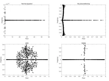

Fig.4.2 Eigenvalue distributions for the case (ii)(n=1024)in Example 4.1
杂志排行

应用数学的其它文章
- Threshold Dynamics of Discrete HIV Virus Model with Therapy
- Solvability for Fractional p-Laplacian Differential Equation with Integral Boundary Conditions at Resonance on Infinite Interval
- Long-Time Dynamics of Solutions for a Class of Coupling Beam Equations with Nonlinear Boundary Conditions
- Existence and Uniqueness of Mild Solutions for Nonlinear Fractional Integro-Differential Evolution Equations
- 基于Markov链的税延型养老保险跨期效用
- 动态投资组合现金次可加风险度量的时间相容性