Remarks on Time-Accurate Adjoint of Quasi-One-Dimensional Euler Equations*

Liang-yuan Tian Lu-cheng JiXin Li

（Beijing Institute of Technology,Beijing,China,E-mail:jilc@bit.edu.cn）

Abstract：For the optimization of turbine equipment, artificial regulation relying on the experience and global optimization are difficult to ensure the optimization efficiency. Thus, local optimization, mainly including the Adjoint method, becomes the mainstream of optimization. The Adjoint method used for steady flow in both external and internal field and unsteady flow in external field has got wide attention and researches. However, in internal field, the research on strictly time- accurate Adjoint optimization is rare. In this paper, the time- accurate Adjoint method for quasi- onedimensional Euler equations is detailed derived and the discretization format is given specifically. Besides, the timeaccurate Adjoint method is carried out in a duct. The gradient distribution compared with the Complex-Variable method shows correctness of the Adjoint equation and numerical discretization, which offers a platform for 3D turbomachinery time-accurateAdjoint optimization research.>For the optimization of turbine equipment, artificial regulation relying on the experience and global optimization are difficult to ensure the optimization efficiency. Thus, local optimization, mainly including the Adjoint method, becomes the mainstream of optimization. TheAdjoint method used for steady flow in both external and internal field and unsteady flow in external field has got wide attention and researches. However, in internal field, the research on strictly time- accurate Adjoint optimization is rare. In this paper, the time- accurate Adjoint method for quasi- onedimensional Euler equations is detailed derived and the discretization format is given specifically. Besides, the timeaccurate Adjoint method is carried out in a duct. The gradient distribution compared with the Complex-Variable method shows correctness of the Adjoint equation and numerical discretization, which offers a platform for 3D turbomachinery time-accurateAdjoint optimization research.

Keywords：Time-Accurate，Quasi-One-Dimensional，Euler Equations，Adjoint Method，Discretization，Gradient Distribution

0 Introduction

As an approach of local optimization,gradient-based algorithm is becoming widespread in the application of aerodynamic shape optimization[1].Gradient-based algorithm relies on the gradient information of the objective function,computed from the sensitivity calculation,to confirm the changes of all design variables,which are determined by the optimal process.Sensitivity calculation offers the necessary gradient messages for the subsequent optimal processes,playing a decisive role in the whole procedure.

The complexity of sensitivity calculation mainly lies in the highly nonlinear characteristics of flow governing equations,which makes the computation cost an important factor.The Adjoint method has an advantage of its calculation cost has nearly no relationship with the number of design parameters,making it a popular method in the optimization of turbomachine.Nowadays,in the field of external flow,both steady and unsteady Adjoint method has been widely used and become mature[2-18].However,for the Adjoint method in internal flow,there is little research on the strict definition of the time-accurate flow.

Considering the quasi-one-dimensional Euler equations describe the flow in an axial symmetry duct,which is the simplest simulation about 3D internal flow,this paper uses quasi-one-dimensional flow as the basis and systematically studies the time-accurate Adjoint method,including the derivation of the Adjoint equation,the discretization format and simulation calibration.The factors of the unsteady flow are detailed compared and the Adjoint field is shown.The final sensitivity distribution is proved accurately enough,giving the experience to develop the time-accurate 3D turbomachineryAdjoint optimization system.

1 Time-Accurate Adjoint Method

1.1 Flow equation

The quasi-one-dimensional flow is governed by Euler Equations[19-21].In a duct of cross-sectionh(x),the time-accurate Euler equation can be expressed as:

where:

Here,ρis the density,υis the velocity,pis the pressure andEis the total energy.

1.2 Object function

The general form of object function used in time-accurate optimization can be written as:

Here,I0andI1are evaluations of the flow field and design parameters.

In equation(2),the first termmeasures the flow fields in a time scale,and the second term,,assesses the flow at a specific time.

1.3 Continuous adjoint equation

The derivation of time-accurate Adjoint equations is similar to steady Adjoint equations’,mainly containing the‘linearization-operation-discretization’ process.In detail,the continuous Adjoint equations of time-accurate quasi-one-dimensional flow can be derived as follows:

1.3.1 Linearization

The highly nonlinear property of flow control equations brings much difficulties on the calculation of the objective function’s gradients.By linearizing the Euler equations,this process is going to simplify the expression of gradients.

According to the perturbation method,when a small perturbΔαis added to the design parameterα,the relative terms in Euler equations can be expressed as:here,the subscript0presents the terms before perturbation.

Combining the Euler equations,equation(4),and ignoring the high order dimensionless,we can get that:

Then:

1.3.2 Numerical operation

This process mainly simplifies the equation(7)and derivates the final expression of continuousAdjoint equation.

Introducing the Lagrange multiplier toδR,expression can be get that:

In equation(8),the following equality relationship should be followed:

Then equation(10)can be expressed as:

As for Euler flow in an axial symmetry duct,in this paper,the object function is firstly chosen as:

Now making a simplified equality that:

Then equation(12)becomes:

Considering the gradient of the objective function:

Combining equation(13)and(14),the expression of gradient can be stated as:

After rearrange the order of each term in equation(15):

The key of the Adjoint method is to eliminate the influence of,so the following equipment relationship should be obeyed.

In the equations above,equation(16-c)contains the demand of equation(16-e),so equation(16-e)can be ignored.As for equation(16-b),the requirement is so difficult that this demand usually can't be satisfied. But whent1=t0+n·T,wherenis natural number andTis period of the flow,meaning that the flow filed must be periodic,the demand of equation(16-b)is easily to be achieved.Under this condition,the demand of equation(16-d),meaning the Adjoint filed att=t0must be zero,is unpractical.

Considering the flow in turbomachine,the flow filed meets the condition of periodicity,and usually the need of evaluating the flow at specific time is unnecessary.Combin-ing the character of flow in turbomachine and the demand of equation(16-b),the normal form of objective function should be:

In this paper,the objective function is re-chosen as:

The remaining terms in equation(15)include:

Introducing the virtual time step in equation(19),then:

Equation(21)is the final form of the continuous Adjoint equation and equation(20)is the boundary condition of continuousAdjoint equation.

Therefore,the gradient of objective function can be gotten as:

1.3.3 Numerical discretization

The task of this process is discretizing equation(21)for the numerical calculation.Detail format will be introduced in chapter 2.2.

2 Numerical Implementation

2.1 Flow solver

In this paper,the time-accurate Euler equations are solved by dual time-stepping method.Therefore,adding the virtual time step in Euler equations is necessary.

The Euler equations above,in this paper,are discretized using a finite-difference,vertex-centered scheme.On the virtual time step,fourth-order Runge-Kutta method is employed as equation(24):

At an interior cell,a central scheme with JST-type artificial dissipation for numerical residual is given as[23]:

where:

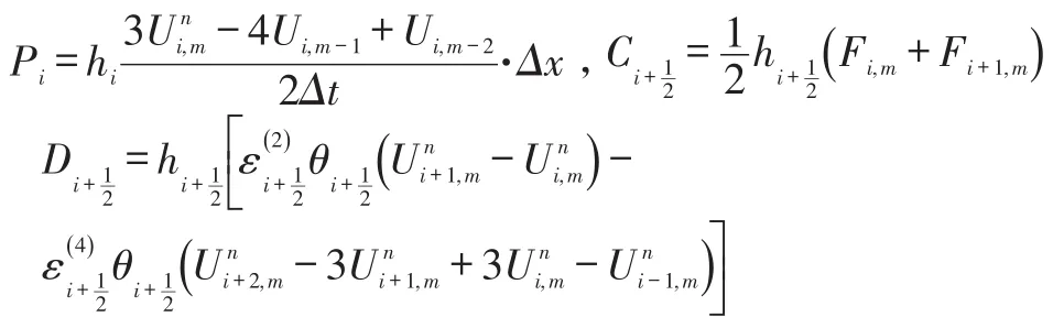
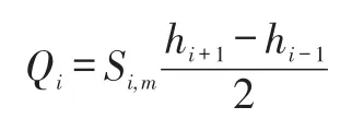
with:

In equations above,the termsUi,m-1andUi,m-2represent the convergent solutions atm-1andm-2physical time levels.

As for the boundary of calculation filed,this paper uses a strongly imposed way.For different flow conditions,such as subsonic or supersonic inlet or outlet conditions,the flow terms at boundary,which should be given before calculation(subscriptbc),are fixed(subscript0),and the except are defined by extrapolation.

where cell indices run from 1 toim.

2.2 Continuous adjoint solver

As mentioned above,the last process dealing with continuous Adjoint method is discretizing,which is to discretize the equation(21)for numerical calculation.

The time-accurate continuous Adjoint equation(21),has a similar form with Euler equations(1).Therefore,the discretization can refer to equation(25).At an interior cell,the numerical discretization can be expressed as:

The numerical residual takes the form:

where:

Except the parameters introduced above,all other terms in equations above are completely the same as those for the flow solver.

One important and obvious difference between the two discretization formats isPiand,reflecting the advancing direction of those two solvers is opposite.

Equation(20)defines the boundary conditions of the continuous Adjoint equation.For flow terms which is constant at boundary,.Therefore,the calculation ofψbcis through extrapolation.But for the other terms at boundaries,,somust be zero,meaning that those adjoint variables are calculated and fixed.

2.3 Discrete adjoint

Compared to the continuous Adjoint method,the discrete Adjoint method uses the flow solver’s discretization before the linearization process in the derivation.It makes that there is no need to discretize the finalAdjoint equation.

Replace theRterm in the previous equation with the discrete form in equation(25)and the sensitivity can then be expressed as:

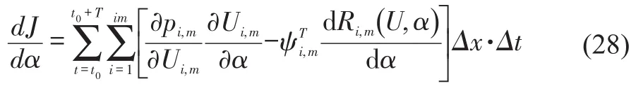
Rearranging the equation(28)to group the coefficient oftogether,the discrete adjoint discretization can be obtained directly.For example,the physical time term in equation(25)is that:

The form of physical time term in equation(28)is that:

Now grouping the coefficient of:

Rearranging the form of equation(31):

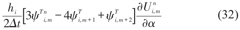
Although equations(29)to(32)are not the whole form ofRi,m,this procedure describes how the discrete Adjoint equations derivate,and confirms the advancing direction of Adjoint discretization is opposite to flow solver.

Finally,the discreteAdjoint discretization format is:

where:

with:

Similar to the continuous Adjoint,except the parameters introduced above,all other terms in equations above are completely the same as the flow solver.

3 Results and Analysis

3.1 Flow field

The duct used in this paper is a transonic converging-diverging nozzle,with a distribution of cross-sectional area[20-22]that:

Total pressure(p0)and total enthalpy(h0)remain constant at inlet and the static pressure(p)at outlet is varied sinusoidally.

Considering the analytical solutions of unsteady Euler equations are difficult to supply,suppose the static pressure at outlet is constant with a value of 1.6,turn off the physical time term in equation(23),and then verify the correctness of numerical discretization of Euler equations.Analytical(derived by the Area-Mach Relation)and numerical solutions(calculated in total 101 grids)of Mach number are shown in Figure(1).Intuitively,the discretization of steady terms in Euler equations are accurate enough.

Fig.1 Distribution of analytic and numerical Mach number

3.1.1 Influence of amplitude of back pressure fluctuation

The impact of amplitude of back pressure fluctuation,depicted in Figure(2),is verified in a range of0＜ε≤0.3,at a fixedω=2,im=101and(meaning total 100 physical time steps in a physical time period).

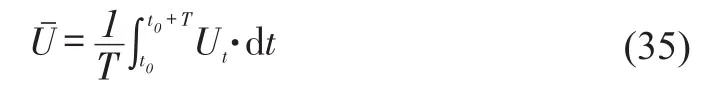
In the flow field schematic diagrams in Figure(2),the black lines represent the steady flow,when the static pressure at outlet keeps unchanged at 1.6.The blue lines show the time-averaged flow,calculated by equation(35).And the red lines present the envelope of unsteady flow.

As shown in Figure(2),with different amplitudes of back pressure fluctuation,all cases take nearly the same number of physical steps to get to the convergent status,while the variation ranges are strongly associated with the amplitude.For the flow fields,the relationships of different phasic flows are almost the same.As the growth of the amplitude,more positions before the shock wave are influenced by the vibration of the static pressure at outlet,and the scope of flow’s variation increases gradually.In the meantime,the differences between time-averaged flow and steady flow are magnified.

3.1.2 Influence of frequency of back pressure fluctuation.

Fig.2 Impact of amplitude of back pressure fluctuation

The frequency of back pressure fluctuation is related to the character frequency of the Euler flow.Calculating the av-erage velocity of steady Euler flow and combining the length of nozzle,we can get the character frequency through equation(36):

Strouhal number is a dimensionless number describing oscillating flow mechanisms in dimensional analysis,which is often given as:

The impact of frequency of back pressure fluctuation is considered by three different frequencies,ω=0.5,ω=2.0andω=4.0,corresponding toSt=0.3,1.1,2.2,at a fixed condition thatε=0.3,im=101and.The influences are drawn in Figure(3),by the same way of Figure(2).

Reconsider the definition of Stroughal number and replace the frequency terms with time in equation(37).

From equation(38),we can say that the Stroughal number can measure the time virtual iteration used to calculate from inlet to outlet and physical time period.Define a virtual procedure as a full process where a data message can transfer from inlet to outlet.So,in other words,with the increase of Stroughal number,in a physical time period,less virtual procedures occur.From this point,Figure(3)can be analyzed.

Fig.3 Impact of frequency of back pressure fluctuation

As the growth ofωandSt,it takes more physical steps or physical time periods to get to the convergent status.Also,intersections between different phasic flow curves are increased and the vibration range of phasic flows are increased.The former phenomenon can be explained by the virtual procedure.The virtual procedures calculation needs to get to the convergent status are relatively constant.With the increase ofSt,to keep the same virtual procedures,more physical periods must be occupied.Also,the increase of frequency augments the value of,making it understandable for the second phenomenon.

3.1.3 Influence of number of time steps in a physical time period.

The number of time steps in a physical time period is also an important factor that influences the time-accurate Euler flow.A physical time period is divided into 100,200 and 300 physical time steps to examine the impact.At a fixed condition ofε=0.3,im=101andω=2.0,the impacts are shown in Figure(4).

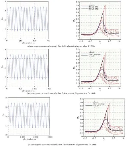
Fig.4 Impact of number of time steps in a physical time period

From the view of discretization,when the total time of a physical time period is fixed,the number of time steps in a physical time period only affects the numerical accuracy of,while the numerical values are approximately equal.So,from Figure(4),we can see that the characteristics of convergence(measured by the periods)and phasic flow are nearly the same.The differences are mainly reflected on the curve shape of phasic flow after the shock wave.To put it in another way,the number of time steps in a physical time period decides the‘grid’in the time level,equal to the concept of spatial mesh.So,the choice of physical time steps should be moderate,preventing the case of inaccuracy or much numerical errors.

3.2 Adjoint field

Combining the analysis in chapter 3.1,the adjoint field is calculated at a fixed condition thatε=0.3,im=101,ω=2.0and.The steady adjoint field(ε=0)is firstly solved and compared with the analytical solutions(derived by Michael B.Giles and Niles A.Pierce)in Figure(5),which proves the correctness of numerical discretization of equation(26)and(28).

Given the fact that the analytical adjoint field of unsteady Euler equations is too complex to derive,the correctness of adjoint distribution is verified not directly but through the correctness of gradient distribution in chapter3.3.The convergence curves and adjoint fields are shown in Figure(6).

From Figure(6),we can see that the differences between results of continuous Adjoint method and discrete Adjoint method are much small,for not only the convergent curve,but also the adjoint curve.The difference between continuous and discrete adjoint is not an emphasis in this research and no more detail comparisons will be done.

Comparing the Figure(4-b)and Figure(6-b),we can find that the adjoint fileds take more physical steps to get to the convergent status.Besides,the vibration of adjoint field,mainly distributed before the shock wave,which is opposite to the flow field,is much severe.Considering the direction of data transport of Adjoint equations,this phenomenon is understandable.Also,more deviations between time-averaged field between steady ones occur,indicating more numerical errors are introduced when calculating the unsteady field with steady state.

3.3 Gradient distribution

In this paper,the Hicks-Henne perturb function is chosen as the parametric model,which is given as:

where:

here,xis the axis position,the subscriptjis the current mesh point,subscriptinmeans the inlet of duct andoutmeans the outlet,Kis the number of design variables.

After thekthdesign variable induces a perturbation,the new area atjthgrid point becomes:

Under the parametric model introduced above,according to equation(15),the gradient distribution of both continuous Adjoint method and discrete Adjoint method can be solved.Meanwhile,in view of the Complex-Variable method is a relatively accurate way while its results are not influenced by the step size of perturbations,this paper uses the sensitivity information calculated by Complex-Variable method to assess the results of Adjoint methods,which is shown in Figure(7).

Fig.5 Distribution ofAdjoint variables

Fig.6 Time-accurateAdjoint iteration curve and fields

Fig.7 Comparison of the gradient distribution

The left picture in Figure(7)describes the gradient distribution at the fix condition whereε=0.3,im=101,ω=2.0and.Noticing that the result of discrete A-djoint method still have relatively large errors from the Complex-Variable method,the gradientdistribution whenε=0.3,im=101,ω=4.0andis given too.As we can see from the right picture in Figure(7),it can be concluded that both the continuous Adjoint method and discrete Adjoint method introduced above is right.Combined with the left figure,from the viewpoint of numerical errors,the continuous Adjoint method is more accurate than the discrete Adjoint method.And on the whole,both types of the Adjoint methods are accurate enough for the optimization.

4 Conclusions

In this study,a detail description of the procedure to obtain the time-accurate adjoint solutions of the quasi-one-dimensional unsteady Euler equations is provided.The derivation of time-accurate continuous Adjoint equations,numerical discretization format of time-accurate Euler Equations,continuous Adjoint equations and discrete Adjoint equations are introduced to offer a platform for time-accurate Adjoint optimization research.

By introducing a perturbation to static pressure at the outlet of duct,the original steady flow turns to unsteady one.This paper systematically studies the influences of perturbance parameters on the character of convergence and flow field.The results show that the frequency and amplitude of perturbation,the physical time steps have remarkable impacts on the flow filed and therefore on theAdjoint field.

In this paper,time-accurate Continuous Adjoint equations of Euler equations are detailed derived and the numerical discretization format of continuous and discrete Adjoint equations is provided.The comparison between steady-state solutions and analytical ones,associating with the comparison of gradient distribution between Complex-Variable method and Adjoint methods,fundamentally proves the correctness ofAdjoint equations and its discretization format.