LIOUVILLE TYPE THEOREM FOR THE STATIONARY EQUATIONS OF MAGNETO-HYDRODYNAMICS∗

Simon SCHULZ

Mathematical Institute,University of Oxford,Woodstock Road,OX2 6GG,Oxford,United Kingdom E-mail:simon.schulz1@maths.ox.ac.uk

Abstract We show that any smooth solution(u,H)to the stationary equations of magnetohydrodynamics belonging to both spaces L6(R3)and BMO−1(R3)must be identically zero.This is an extension of previous results,all of which systematically required stronger integrability and the additional assumption∇u,∇H∈L2(R3),i.e., finite Dirichlet integral.

Key words Liouville theorem;Caccioppoli inequality;Navier-Stokes equations;MHD

1 Introduction

Liouville type theorems arise naturally when considering the regularity of solutions to the incompressible Navier-Stokes equations.Development in this direction has been led most notably by Chae,Nadirashvili,Seregin,and Šverák(cf.[2,5,7]).Intimately tied to the Navier-Stokes equations are the equations of magneto-hydrodynamics(MHD).The latter system models the motion of an incompressible fluid whose velocity field is a ff ected by magnetic interactions,e.g.,the movement of a magnetized plasma.

Liouville type theorems were known to hold for the MHD system,as demonstrated by the works[3,9].In[3],Chae proved that if a smooth solution of the stationary MHD equations is bounded in L3(R3)and has finite Dirichlet integral,then it is identically zero.Later,in[9],Zhang-Yang-Qiu proved that if a smooth solution of the stationary MHD equations is bounded inand has finite Dirichlet integral,then it is also identically zero.So far,no result exists without the finite Dirichlet integral assumption

The focus of this paper is to obtain a Liouville theorem for the equations of stationary MHD without the need for finite Dirichlet integral,and with only an L6(R3)integrability criterion.To this end,we closely follow the scheme outlined by Seregin in[7].In using this approach,we also reprove the original results in[3]and[9]without the requirementAlthough many of the estimates in this work are identical to those in[7],we go through them in detail for the sake of making this paper self-contained.

2 Preliminaries

In what follows we employ the method of Seregin in[7],which first and foremost involves proving a Caccioppoli type inequality.Although Seregin’s paper is concerned with the stationary incompressible Navier-Stokes equations,his proof makes a similar Caccioppoli type inequality hold for the equations of magneto-hydrodynamics.In light of this,we structure our paper in the same way as was done in[7].

Below are the equations of stationary MHD.As per usual,u is the velocity of the fluid and H is the magnetic field,

De finition 2.1We say thatif there exists a skew-symmetric tensor d∈BMO(R3)such thatfor i=1,2,3.

Remark 2.2Observe that the requirement that a vector be the divergence of a skewsymmetric tensor is “equivalent” to this vector being equal to a curl.Formally,we have

Remark 2.3If d∈BMO(R3),then

for each 1≤s<∞.Here,[d]x0,rdenotes the mean value of d in the ball B(x0,r).We recurrently use the finiteness of this quantity in our later estimates.

We begin by showing the following theorem.

Theorem 2.4Let(u,H)be a smooth solution of system(2.1)with u,H∈BMO−1(R3).If we additionally require that u,H∈Lq(R3)for q∈(2,6),then u≡0 and H≡0.

Note that the above covers the cases explored by Chae in[3]and Zhang-Yang-Qiu in[9].However,unlike them,we do not additionally requireA supplementary argument then yield the result claimed in the abstract,which is contained in the theorem underneath.

Theorem 2.5Let(u,H)be a smooth solution of system(2.1)with u,H∈BMO−1(R3).If we additionally require that u,H∈L6(R3),then u≡0 and H≡0.

3 Proof of the Main Results

3.1 Caccioppoli Type Inequality

Much like in[7],we have at the heart of our proof a Caccioppoli type inequality,which we develop in this portion of the paper.We state this inequality below.

Lemma 3.1Let(u,H)be a smooth solution to system(2.1)with u,H∈BMO−1(R3),and let v:=u+H.Then the Caccioppoli type inequality

holds for any ball B(x0,R)⊂R3,any constant v0∈R3,and any s>2.

ProofBegin by adding the two evolution equations together to obtain(

Note that,since both u and H are in BMO−1(R3),we know that their di ff erence u−H and v are also BMO−1vector fields.In particular,we know that there exists a skew-symmetric tensor d∈BMO(R3)such that u−H=divd.

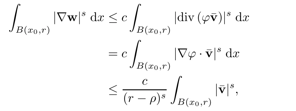
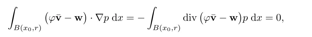
Take an arbitrary ball B(x0,R)in R3and a non-negative cut-o fffunctionwith the properties:ϕ(x)=1 in B(x0,ρ),ϕ(x)=0 outside of B(x0,r),andfor any R/2≤ρ

Now,consider the following Dirichlet problem

Since the right-hand side of the equation integrates to zero(by the divergence theorem)and is locally integrable,we deduce from Theorem 3.6 in Chapter 1 of[6](or from[1])that there existssolving the above,and for which the following inequality holds for 1

here c=c(s)and is independent of x0and R.

Next,we follow the bounds as in[7],i.e.,we test the second equation in(3.2)againstto get

We denote the previous integrals by I1,···,I4.

Remark 3.2The term involving∇p has vanished,sinceis divergence-free and

where the boundary term has vanished due to the compact support of our test function.

Now we bound the numbered integrals I1,···,I4,

So,we have

Similarly,

Note that we have implicitly assumed that s>2.

For I3and I4we need to use the skew-symmetry of d.

For the fourth integral

In total,we have

Applying a weighted Cauchy-Schwarz inequality,we obtain

Suitable iterations then give the following Caccioppoli type inequality

as required.

Remark 3.3The positive constant c is independent of x0and R,and depends only on s.

3.2 The Proof of Theorem 2.4

The proof of Theorem 2.4 rests entirely on the observation that we can make the exponent 1−6/s negative in the Caccioppoli type inequality(3.1).In view of this,we present our proof.

Proof of Theorem 2.4Suppose u,H ∈ Lq(R3)for 20,so by choosing v0=0 the Caccioppoli type inequality(3.1)now reads

By taking the limit as R→∞we recover.This implies that v is constant,but since v∈Lq(R3),we know that this constant must be zero.Hence

Using this relation,we know from the first evolution equation for u in(2.1)that(

Once again,we obtain

so choosing u0=0 we get

Taking the limit as R→∞we recover,which concludes the proof of the theorem. ?

3.3 The Proof of Theorem 2.5

In the case where s=6 we cannot argue as we did previously.Putting s=6 and v0=0 in(3.1)yields

Hence,passing to the limit R→∞gives the reverse Sobolev inequality

This is not particularly useful in itself,and does not readily produce a reverse Sobolev inequality for the individual vector fields u and H.Instead,one can pick s=3 and v0=[v]x0,Rwith the aim of constructing an inequality between maximal functions.This is precisely how the proof of Theorem 2.5 runs,which we elaborate on in the next few paragraphs.

Proof of Theorem 2.5Firstly recall the Gagliardo-Nirenberg type inequality

Now choose s=3 and v0=[v]x0,Rin the Caccioppoli type inequality(3.1),and couple this with(3.5)to obtain the reverse Hölder inequality

where c is independent of x0and R,as per usual.

be its Hardy-Littlewood maximal function.Now the reverse Hölder inequality(3.6)reads

From the maximal function inequality in Lp(R3)for p>1(c.f.[8]),we know that there exists a universal constant c0>0 such that

where the last inequality is exactly(3.4).Thus we have shown that bothand its maximal function Mh43are L1(R3)functions,which is only possible if h≡0(c.f.[8]).This implies that v is constant,thus once again we arrive at

We now show that we must have u≡0.Making use of the relationas we did in the proof of Theorem 2.4,we recover(3.3)and the Caccioppoli type inequality

Picking q=6 and u0=0 we recover

as expected.Selecting q=3 andand using the same strategy as before,we arrive at the maximal function inequality

AcknowledgementsThe author wishes to thank Gui-Qiang Chen and Gregory Seregin for useful discussions.