LOW MACH NUMBER LIMIT OF A COMPRESSIBLE NON-ISOTHERMAL NEMATIC LIQUID CRYSTALS MODEL∗

樊继山

Department of Applied Mathematics,Nanjing Forestry University,Nanjing 210037,China E-mail:fanjishan@njfu.edu.cn

Fucai LI(栗付才)†

Department of Mathematics,Nanjing University,Nanjing 210093,China E-mail: fli@nju.edu.cn

Abstract In this paper,we study the low Mach number limit of a compressible nonisothermal model for nematic liquid crystals in a bounded domain.We establish the uniform estimates with respect to the Mach number,and thus prove the convergence to the solution of the incompressible model for nematic liquid crystals.

Key words compressible non-isothermal liquid crystals;bounded domain;low Mach number limit

1 Introduction

Let Ω⊂R3be a bounded smooth and simply connected domain,and n be the unit outward normal vector of the boundary ∂Ω.We consider the following simpli fied version of Ericksen-Leslie system modeling the hydrodynamic flow of compressible nematic liquid crystals

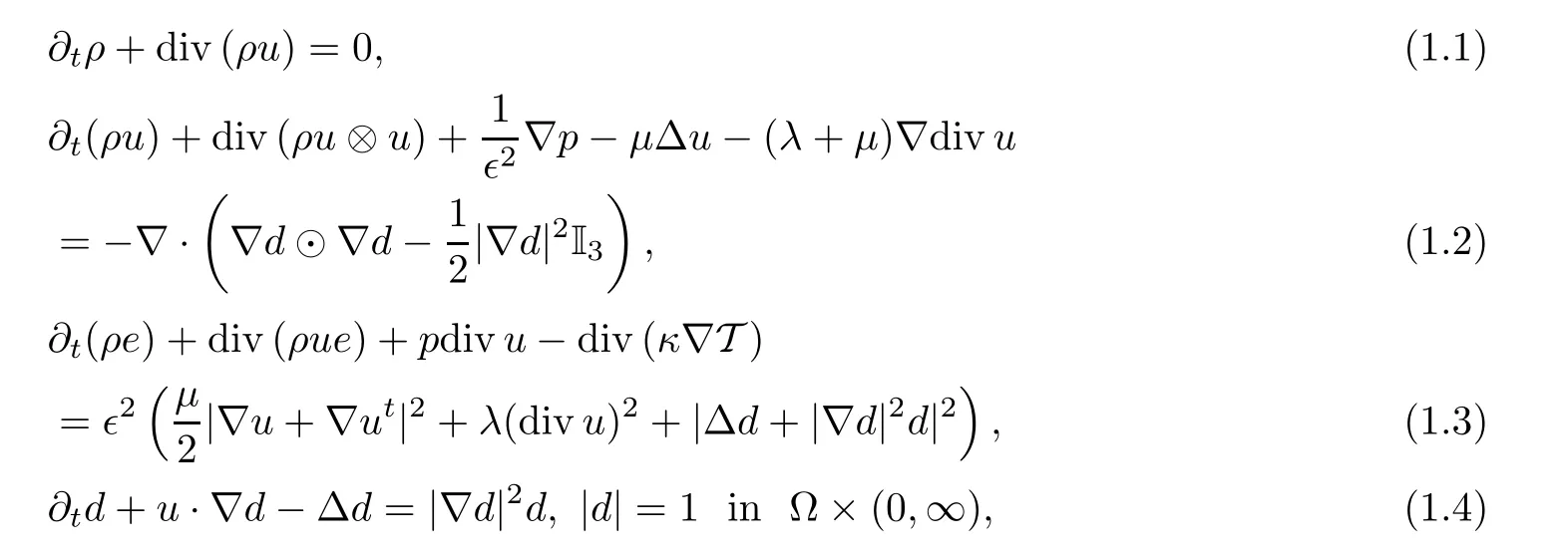
here ρ,u,T denote the density,velocity and temperature of the fluid,respectively,and d represents the macroscopic average of the nematic liquid crystals orientation field.e:=CVT is the internal energy and p:=RρT is the pressure with positive constants CVand R.The viscosity coefficients µ and λ of the fluid satisfy µ >0 and λ +µ ≥ 0. The parameter ǫ>0 is the compressibility parameter which is proportional to the Mach number(see[18,25]),and κ >0 is the heat conductivity coefficient.The symbol∇d⊙∇d denotes a matrix whose(i,j)th entry is ∂id∂jd,I3is the identity matrix of order 3,and it is easy to see that denotes the transpose of vector u.

Recently,Guo,Xi and Xie[12]studied the global existence of small smooth solutions to the system(1.1)–(1.4)in the whole space R3.When the term|∇d|2in(1.3)and(1.4)is replaced by the Ginzburg-Landau approximation termGuo,Xi and Xie[13]showed the existence of global weak solutions to the problem(1.1)–(1.6)with some structure assumptions.In[8],we,collaborated with Nakamura,established the local well-posedness of strong solutions to the problem(1.1)–(1.6).

When the prescribed fluid is incompressible,i.e.,divu=0,the system(1.1)–(1.4)is reduced to the incompressible non-isothermal models with the Ginzburg-Landau approximation term introduced by Feireisl et al.[9].Feireisl,Rocca,and Shimperna[10]established the existence of global-in-time weak solutions for a similar incompressible non-isothermal Models.Gu,Fan,and Zhou[11]obtained some regularity criteria for the model introduced in[10].Li and Xin[19]obtained the global existence of weak solutions to an incompressible non-isothermal nematic liquid crystal system on the torus T2.

We remark that there are a lot of work on the barotropic models of compressible nematic liquid crystals,among others,see[14,20]on the local well-posedness of strong solutions,[4,15]on the regularity criteria,[16,17,21]on the global existence of weak solutions,and[6,24,27]on the low Mach number limit.

The purpose of this paper is to deal with the low Mach number limit of the compressible non-isothermal model(1.1)–(1.4)in a bounded domain with the boundary condition(1.5)for well-prepared initial data.In the following,we introduce the new unknowns σ and θ,which denote the variations of the density ρ and the temperature T,respectively,by

Then the problem(1.1)–(1.6)can be rewritten as

De finition 1.1

Remark 1.2To simplify the statement, ∂tσ(0)is indeed de fined by −div(σ0u0)divu0through the density equation,andσ(0)is given recursively by applying ∂tto(1.7)in the same manner.Similarly,we can de fine ρt(0),ρtt(0),etc.

A local existence result for the problem(1.7)–(1.12)in the following sense can be shown in a similar way to those in[8].Thus we omit the details of the proof.

Proposition 1.3(Local existence)Let 0<ǫ≤1.Suppose that the initial dataandsatisfy 1+≥δ,1+≥0 for some constant δ>0,and

Then there exists a positive time Tǫ>0 such that the problem(1.7)–(1.12)has a unique solution(σǫ,uǫ,θǫ,dǫ),satisfying that for k=0,1,2,

The main result of this paper is stated as follows,which shows the uniform estimates of strong solutions to(1.7)–(1.12)with respect to the Mach number ǫ,and the corresponding low Mach number limit.

Theorem 1.4Assume that(σǫ,uǫ,θǫ,dǫ)is the solution obtained in Proposition 1.3,where the initial datasatis fies

Then there exist positive constants T0and D such that(σǫ,uǫ,θǫ,dǫ)satis fies the uniform estimates

here D0,T0,and D are constants independent of ǫ.Furthermore,(σǫ,uǫ,θǫ,dǫ)converges to(σ,u,θ,d)in certain Sobolev space as ǫ→ 0,and there exists a function π(x,t)such that(u,d,π)∈ C([0,T0];H2)solves the initial-boundary value problem of the incompressible model

of nematic liquid crystals:

where u0,d0are the weak limits ofandrespectively,in H2(Ω)and H3(Ω)with divu0=0 in Ω.

De finition 1.5

We can prove

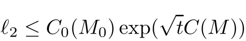
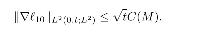
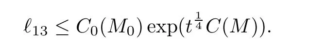
Theorem 1.6Let Tǫbe the maximal time of existence for the problem(1.7)–(1.12)in the sense of Proposition 1.3.Then for any t∈ [0,Tǫ),we have that

for some given nondecreasing continuous functions C0(·)and C(·).

In the following proofs,we will use the Poincaré inequality[22]

for any w ∈H1(Ω)with w·n=0 or w×n=0 on ∂Ω.

We will also use the following two inequalities[3,26]

for any w ∈Hs(Ω)and s≥1.

2 Proofs of Theorems 1.4 and 1.6

This section is devoted to the proofs of Theorems 1.4 and 1.6.We use some ideas developed in[1,5,7,23].First,by taking the similar arguments to that[1,7,23],we know that in order to prove

it suffices to show inequality(1.16).Next,based on the uniform estimates of the solutions,we can prove the convergence results in Theorem 1.4 by applying the Arzelà-Ascoli’s theorem

Below we shall drop the superscript“ǫ”of ρǫ,σǫ,uǫ,θǫ,dǫ,and Mǫ,for the sake of simplicity.We shall denote∂tu by ut,et al..

First,by the same calculations as that in[5],we get

Next,it is easy to see that

Similarly,we infer that

Now we are in a position to give estimates of d.

Lemma 2.1

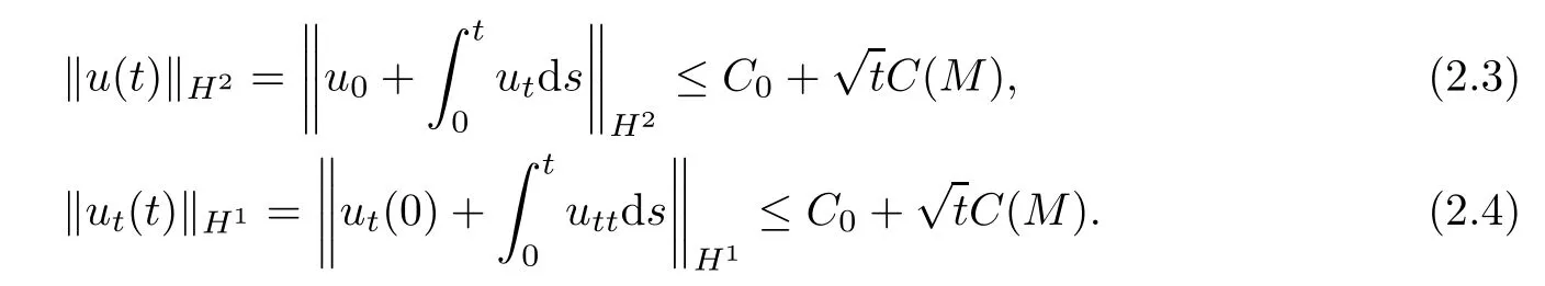
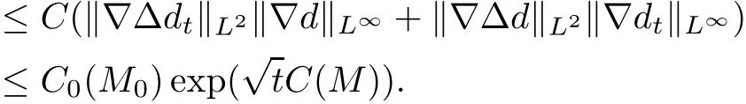
ProofBy the H4-theory of Poisson equation,it follows from(1.10),(2.3)and(2.7)that

whence

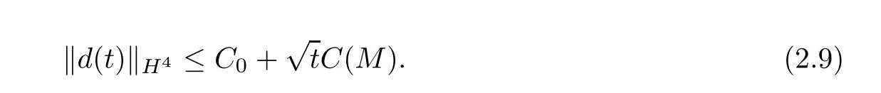
Integrating the above estimates over(0,t),we have

By the H3-theory of Poisson equation,it follows from(1.10),(2.10),(2.3),(2.4),and(2.7)that

This completes the proof of Lemma 2.1.

Lemma 2.2For any 0≤ t≤ min{Tǫ,1},we have

ProofTaking rot to(1.8),using(2.8),(2.2),(2.3),and(2.4),we observe that

This proves(2.12).

Lemma 2.3For any 0≤ t≤ min{Tǫ,1},we have

ProofSince we have rot2u·n=0 on ∂Ω×(0,∞)([2]),by using(1.17)and(2.12),we easily get(2.13). ?

Lemma 2.4For any 0≤ t≤ min{Tǫ,1},we have

ProofDenoting the voracity ω:=rotu,it is easy to compute that

where

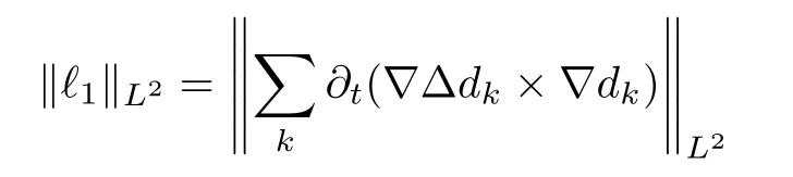
Compared to that in[5],here ℓ1is the only new term.

We bound ℓ1as

Then by taking the same calculations as that in[5]and(2.13),we have

Here we used the same estimate

as in[5]and thus we omit the details here.This proves(2.14).

Using(2.4),(2.16)and integration by parts,we find that

Next,we will estimate the spatial derivatives of(σt,ut,θt).So an application of the operator∂tto the system(1.7)–(1.9)leads to

Lemma 2.5For any 0≤ t≤ min{Tǫ,1},we have

ProofTesting(2.19)by∇divut,we observe that

It was proved in[5]that

We bound the only new term ℓ4as

Applying similar arguments to(2.20)yields

It was proved in[5]that

We bound the only new term ℓ6as

On the other hand,it was proved in[5]that

Summing up(2.22),(2.23)and(2.24),we arrive at(2.21).

Next,we show the crucial estimates for k∇2σ(t)kL2and k∇2divukL2(0,t;L2).

Lemma 2.6For any 0≤ t≤ min{Tǫ,1},we have

ProofApplying ∂ito(1.8),testing by ∂i∇divu,we obtain

It was proved in[5]that

We bound the only new term I8as

To cancel the singular term in(2.26),we apply ∂i∇ to(1.7)and test by R(∂i∇σ + ∂i∇θ)and integrate to get

by the same calculations as that in[5].

Inequalities(2.26)and(2.27)yield(2.25).

Lemma 2.7For any 0≤ t≤ min{Tǫ,1},it holds that

ProofDue to(1.7)and(1.9),we discover that

where

Applying∇to(2.29),we have

It was proved in[5]that

It is easy to deduce that

This proves(2.28).

Finally,we estimate σtt,utt,and θttin order to close the energy estimate.

Lemma 2.8For any 0≤ t≤ min{Tǫ,1},we have

ProofFirst,applyingto(1.7),testing by Rσtt,we have

by the same calculations as that in[5].

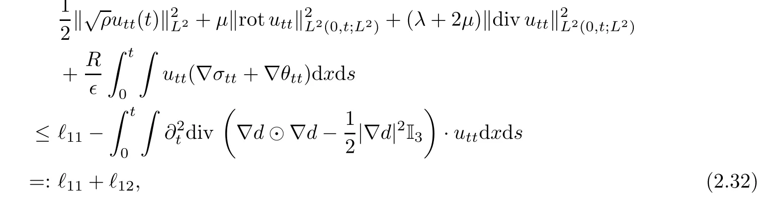
where

It was proved in[5]that

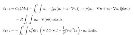
We bound the only new term ℓ12as

where

It was proved in[5]that

We bo

und the only new term ℓ14as follows

Inequalities(2.31),(2.32)and(2.33)gives to(2.30).

By collecting all above estimates together,it is easy to obtain inequality(2.1).Thus the whole proof is completed.