Recurrent 3D attentional networks for end-to-end active object recognition

M in Liu ,Yifei Shi,Lintao Zheng,Kai Xu (),Hui Huang,and Dinesh M anocha

Abstract Active vision is inherently attention-driven:an agent actively selects views to attend in order to rapidly perform a vision task while improving its internal representation of the scene being observed.Inspired by therecent successof attention-based models in 2D vision tasks based on single RGB images,we addressmulti-view depth-based activeobject recognition using an attention mechanism,by use of an end-toend recurrent 3D attentional network.The architecture takes advantage of a recurrent neural network to store and update an internal representation.Our model,trained with 3D shape datasets,is able to iteratively attend the best views targeting an object of interest for recognizing it.To realize 3D view selection,we derive a 3D spatial transformer network.It is dif ferentiable,allowing training with backpropagation,and so achieving much faster convergence than the reinforcement learning employed by most existing attention-based models. Experiments show that our method,with only depth input,achieves state-of-the-art next-bestview performance both in terms of time taken and recognition accuracy.

Keywords active object recognition;recurrent neural network;next-best-view;3D attention

1 Introduction

Active object recognition plays a central role in robotoperated autonomous scene understanding and object manipulation.The problem involves online planning of the views used by a visual sensor on a robot for greatest accuracy and conf idence in object recognition.This is also referred to as the next-best-view(NBV)problem for active object recognition. Recently,3D object recognition has advanced greatly thanks to the rapid development of 3D sensing techniques(e.g.,depth cameras)and the proliferation of 3D shape repositories.Our work adopts a 3D geometric data-driven approach,in a setting of 2.5D depth acquisition.

Most existing works on view selection are based on the paradigm of information theoretic view evaluation,e.g.,Refs.[1,2].For example,from a set of candidates,the view maximizing the mutual information between observations and object classes is selected.Such methods often present two issues.Firstly,to estimate the mutual information,unobserved views must be sampled and the corresponding data must be synthesized from a learned generative model,making view estimation inef ficient[3].Secondly,the object recognition model is typically learned independently of the view planner,although the two are really coupled in an active recognition system[4].

Some works formulate active recognition as a reinforcement learning problem,to learn a viewing policy under various observations. In particular,a few recent works have attempted end-to-end reinforcement learning based on recurrent neural networks[4–6].Applying a learned policy appears to be much more ef ficient than sampling from a generative model.However,these models are known to be hard to train,with dif ficult parameter tuning and relatively long training time[7].Moreover,the success of these methods highly depends on the handdesigned reward functions.

The recent development of attention-based deep modelshasled to signif icant successin 2D vision tasks based on RGB images[7,8].Attention-based models achieve both ef ficiency and accuracy by focusing the processing only on the most informative parts of the input with respect to a given task.Information gained from dif ferent f ixations is integrated into an internal representation,to approach thedesired goal and guide future attention.Such a mechanism,being both goal-directed and stimulus-driven[9],f its well to the problem setting of active recognition,accommodating object recognition and guided acquisition in a unif ied optimization framework.

However,the popular formulation of attention models based on recurrent neural networks[7]suf fers from the problem of non-dif ferentiable recognition loss over attention locations,making network optimization by backpropagation impossible. To make it learnable,training is often turned into a partially observable Markov decision process(POMDP),which comes back to reinforcement learning. The recently introduced dif ferentiable spatial transformer networks(STNs)can be used to actively predict image locations for 2D object detection and recognition[10].Motivated by this,we opt to use STN units as our localization networks.

However,extending standard STNsto predict views in 3D space while keeping their dif ferentiability is non-trivial.To facilitate the backpropagation of loss gradient from a 2.5D depth image to 3D viewing parameters,we propose to parameterize the depth value at each pixel(x,y)in a depth image over the parameters of the corresponding view(θ,ϕ):d(x,y)=f(θ,ϕ),through a ray casting based depth computation at each pixel.Our attention model provides ef ficient view planning and robust object recognition,as demonstrated by our experimental evaluations.Our work contains two main technical contributions:

•A 3D attentional architecture that integrates RNN and STN for simultaneous object recognition and next-best-view(NBV)selection.

•A dif ferentiable extension of STN for view selection in 3D space,leading to an end-to-end attentional network which can be trained ef ficiently.

2 Related work

Active object recognition has a rich literature in robotics,vision,and graphics(see surveys such as Refs.[11,12]). We provide a brief review of 3D object recognition,especially active methods(categorized into information theoretic and policy learning approaches).We then discuss some recent attempts on end-to-end learning for NBV selection.

2.1 3D object recognition

One of the most popular methods for 3D object recognition is directly deploying deep learning on point sets[13,14],but one shortcoming of these works is that point features are treated independently.Based on pioneering work,the Attentional ShapeContextNet[15],which connects shape contexts with convolutional neural networks(CNNs),is able to represent local and global shape information,and achieve competitive results on benchmark datasets.Inspired by image classif ication using CNNs,view-based methods for 3D object recognition have performed best so far.Multiview CNN[3]renders a 3D shape to gray images from dif ferent views,uses a CNN to extract features for each rendered image,and aggregates features from all rendered images with max pooling.A hierarchical view-group-shape architecture is proposed in Ref.[16]aiming to treat each view discriminatively,while all views are treated equally in Ref.[3].Impressive improvement is gained in Ref.[16],but it still needs to evenly sample several views before testing,which means all views are f ixed when testing.This kind of method is not suitable for certain scenarios,such as the robot-operated NBV problem,which always tries to achieve the highest accuracy with as few as possible views.

2.2 Information theoretic ap p roaches

Information theoretic formulation represents a standard approach to active vision problems.The basic idea is to quantify the information gain of each view by measuring mutual information between observations and object classes[1],entropy reduction of object hypotheses[17],or decrease in belief uncertainty about the object that generated the observations[18].The optimal views are those which are expected to provide the maximal information gain.The estimation of information gain usually involveslearning a generativeobject model(likelihood or belief state)so that the posterior distribution of object class under dif ferent views can be estimated.Dif ferent methods have been utilized in estimating information gain,such as Monte Carlo sampling[1],Gaussian process regression[2],and reinforcement learning[19].

2.3 Policy learning ap p roaches

Another lineof research seeksto learn viewing policies.The problem is often viewed as a stochastic optimal control one and cast as a partially-observable Markov decision process.In Ref.[20],reinforcement learning is utilized to of fline learn an approximate policy that maps a sequence of observations to a discriminative viewpoint.Kurniawati et al.[21]employed a pointbased approximate solver to obtain a non-greedy policy of fline.In contrast to of fline learning,Lauri et al.[22]attempted to apply Monte Carlo tree search(MCTS)to obtain an online active hypothesis testing policy for view selection.Our method learns and compiles viewing policies into the hidden layers of an RNN,leading to a high-capacity view planning model.

2.4 End-to-end learning approaches

The recent rapid development of deep learning models has aroused the interest of end-to-end learning of active vision policies[23]. Malmir et al. [24]used deep Q-learning to f ind the optimal policy for view selection from raw images.Our method shares similarities with the recent work of Wu et al. [3]in taking 2.5D depth images as input and 3D shapes as training data.They adopted a volumetric representation of 3D shapes and trained a convolutional deep belief network(CDBN)to model the joint distribution over volume occupancy and shape category.By sampling the distribution,shape completion can beperformed based on observed depth images,over which virtual scanning is conducted to estimate the information gain of a view.Unlike their method,our attention model is trained of fline,so no online sampling is required,making it ef ficient for online active recognition.The works of Jayaraman and Grauman[4],Xu et al.[5],and Chen et al.[6]are the most closely related to ours.Compared to MV-RNN[5],VERAM[6]explicitly integrates view conf idence and view location constraints into the reward function,and deploys strategies for view enhancement.In these methods,the recognition and control modules are jointly optimized based on reinforcement learning.We employ spatial transformer units[10]as our locator networks to obtain a fully dif ferentiable network.

2.5 Spatial transformer networks

A spatial transformer is a dif ferentiable samplingbased network,which givesneural networkstheability to actively transform the input data,without any spatial supervision in training.Generally,a spatial transformer is composed of a localization network and a generator.An STN achieves spatial attention by f irst passing the input image into a localization network which regresses the transformation,and then generating a transformed image using the generator.The transformed image is deemed to be easier to recognize or classify,and thus more suitable for the desired task.

An STN is a good f it to our problem setting.Due to its dif ferentiability,it enables end-to-end training with backpropagation,making the network easier to learn.It is relatively straightforward to employ for object localization in the image of a given view.However,when using it to predict views in 3D,we face the problem of non-dif ferentiable pixel depth values over viewing parameters,which is addressed by our work.

3Approach

We f irst provide an architectural overview of our recurrent attentional model,followed by detailed description of the individual parts.We also provide details of the loss function,model training,and inference.

3.1 Architecture overview

Figure 1 shows the architecture of our recurrent attentional model.The main body of the model is a recurrent neural network(RNN)for modeling the sequential dependencies between consecutive views.In our setting,the 3D shape is located at the center of a sphere with f ixed radius(see Fig.2),and at each time step,the model f irst takes a view(parameterized in the local spherical coordinate system)as input,generates depth images using ray casting and extracts features from the depth images.Then the model amalgamates information of past views,makes a prediction of the categorical label,and produces an update to the current view for future observation.To do so,we embed three parts into the RNN:a depth layer(DL)for generating depth images of objects,a 3D spatial transformer network(3D-STN)for regressing the update to the current view for the shape,and a shape classif ier(SC)for depth-based object recognition.

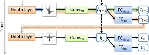
Fig.1 Our recurrent attentional model.The dashed arrows indicate information f low across time steps while the solid ones represent that within a time step.The bold arrows underline the data f lows of the three subnetworks,i.e.,depth layer(DL,blue),3D spatial transformer networks(3D-STN,orange),and shape classif ier(SC,green).

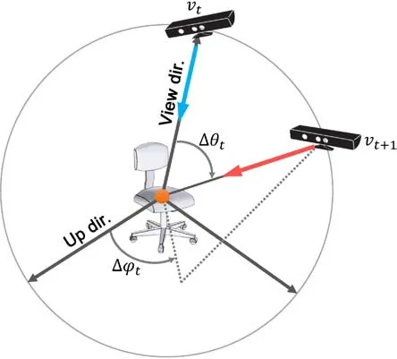
Fig.2 The viewing sphere around the object being recognized.The view at the next time step,v t+1,is parameterized in the local spherical coordinate system based on the current view v t.

Our approach works as follows.Given a current view of an object,it f irst uses a ray casting algorithm to generate a depth image,which is fed into a stack of convolutional layers(Conv2D)for feature extraction.The extracted features are aggregated with those extracted from previous views,with the help of the RNN hidden layers.The aggregated features are then used for classif ication and predicting theupdateto the current view,with the fully connected layers FCclassand FCloc,respectively.With the predicted update to the current view,a next-best-view(vt+1=vt+∆vt)can be obtained.Using vt+1,a new depth image can be generated,which serves as the input at the next time step.

As shown in Fig.1,DL is a single layer subnetwork.3D-STN encompasses the convolutional layers Conv2Dand the fully connected layers FCloc.SC is composed of Conv2Dand FCclass,which is a standard convolutional neural network(CNN)classif ier.Moreover,the convolutional layers are shared by the SC and the 3D-STN.

In order to make our attentional network learnable,we require the generated depth image to be dif ferentiable with respect to the viewing parameters.A basic assumption behind the parameterization of depth values in terms of viewing parameters and the intersection point is that the intersection point does not change when the view change is small,so the f irstorder derivative with respect to viewing parameters can be approximated by keeping the point f ixed.Details are provided in Section 3.2.2.

3.2 Dep th layer for d ep th image generation

The depth layer(DL)is a critical part of our model,both for depth image generation and loss backpropagation.With loss backpropagation,this layer allows us to build up an end-to-end trained deep neural network.During forward propagation,we use ray casting to generate depth images,and record every hit point position on the surface of shapes into a table,which is used in backpropagation.During backpropagation,we f ill the gap between depth images loss gradient and camera views loss gradient.

3.2.1 Ray casting

Ray casting is used to solve the general problem of determining the hit points of a shape intersected by a ray.As illustrated in Fig.3,a view is represented by(R,θt,ϕt),the radial distance to the shape center,polar,and azimuthal angle,respectively.In this spherical coordinate system,R is a constant,and the view direction points to the shape’s center,which is also the origin of the spherical coordinate system.(R,θt,ϕt)can be easily transformed into Cartesian coordinates(Xv,Yv,Zv)by using Eq.(1),where(θt,ϕt)can be obtained by Eq.(2).

As shown in Fig.3,a projection plane lies between the viewpoint vtand the shape.m is the intersection point of the viewing line and the projection plane.For ray casting,we need two points(or one point together with a direction).The position of vtcan be directly computed by Eq.(1).However,f inding position of m is not straightforward.To make things simpler,we use a specif ic setting as follows:when θt=0,the position of vtis(0,0,R),the up direction of the camera is set parallel to the X-axis of spherical coordinate system,and the origin of pixel coordinates is at(0,0,R−f),where f is the focal length of the camera.To go from projection coordinates to pixel coordinates,the camera intrinsic matrix should be applied.If we have a position(um,vm)in pixel coordinates,the projection coordinates(xm,ym)can be calculated by

where d x,d y is a single pixel length along the x-and y-axes of projection coordinates,u0,v0represents the principal point,ideally at the center of the depth images,and the skew coef ficient between x-and y-axes is set to 0.Since we have a predef ined up direction for the camera,we can compute the world coordinate position of each pixel in the projection plane. When vtis located in(R,θt,ϕt),we just apply two rotation matrices to get the new Cartesian coordinate position of each pixel,the f irst rotation beingθtaround the Y-axis,and the second beingϕtaround the Z-axis.

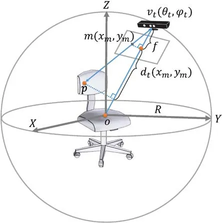
Fig.3 Given a view v t=(θt,ϕt),the depth value of a pixel d t(x m,y m)in the corresponding depth image is parameterized with repsect to the view parameters and the position of the intersection point,p,computed by ray casting.

For each pixel in the projection plane,we can form a ray from vtto m,and the extension of this ray will hit or miss the shape surface.Using a ray casting algorithm,we can get the position(Xp,Yp,Zp)of the hit point(p)on the shape surface(if hit)and the hit distance(Dvp)between the start point(vt)and hit point(p).As shown in Fig.3,if a ray hits the shape,the depth value of the related pixel is represented by dt(xm,ym).The distance between vtand p is calculated by Eq.(4).Using similar triangles gives Eq.(5).We use a table to record all hit points and their related pixels.

3.2.2 Backpropagation

Backpropagation through the depth layer computes loss gradients of input(∆θt−1,∆ϕt−1),given loss gradients of output(depth image). During backpropagation,each pixel will be given a∂loss/∂dt.We obtain the depth value dt,and the hit point position(Xp,Yp,Zp)(which can be directly retrieved from the recorded table),so∂loss/∂∆θt−1and∂loss/∂∆ϕt−1in Eq.(7)can be calculated along with Eqs.(1),(2),(4),(5),and(6).

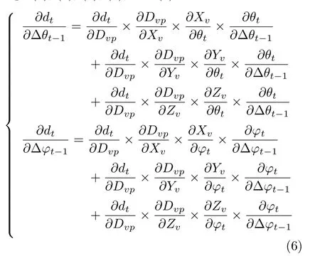
Each pixel of the depth image will be given a∂loss/∂∆θt−1and∂loss/∂∆ϕt−1.We just average all∂loss/∂∆θt−1and∂loss/∂∆ϕt−1to get the f inal loss gradients of(∆θt−1,∆ϕt−1).

3.3 3D-STN for view selection

Given an input depth image,the goal of 3D-STN is to extract image features,and regress the 3D viewing parameters of the update to the current view(∆θt,∆ϕt)with respect to the recognition task.The 3D-STN comprises two subnetworks:Conv2Dand FCloc.During forward passes,Conv2Dtakes the depth image dtas input and extracts features.Using the features,FClocoutputs the update to the current view.The viewing parameter is parameterized in the local spherical coordinate system based on the current view vt(θt,ϕt)(see Fig.2),and represented as a tuple(∆θt,∆ϕt).Note that the viewing parameters do not include radius(R),since R is set to be a constant.

Specif ically,the convolutional network Conv2Df irst extracts features from the depth image output by depth layer:

where W2DConvare the weights of Conv2D.These features are amalgamated with those of past views stored in the RNN hidden layer ht−1:

where g(·)is a nonlinear activation function.Wihand Whhare weights for input-to-hidden and hiddento-hidden connections,respectively.The aggregated features in htare then used to regress the update to the current view:

3.4 Shap e classif ier for object recognition

The depth image output by the depth layer at each timestep ispassed into a shapeclassif ier(SC,Conv2D+FCclass)for class label prediction.Note that the classification is also based on the aggregated features of both current and past views:whereare the weights of.

3.5 Loss function

We employ cross-entropy loss to train our model.Cross-entropy loss measures the performance of a classif ication model whose output is a probability value between 0 and 1.Our loss function is

where k is the number of classes,y is a binary indicator indicating whether classlabel c isthecorrect classif ication for current observation o,and p is the predicted probability that observation o is of class c.

3.6 Training and inference

To make the training more ef ficient,we decompose our training into two parts and tune their parameters separately:(1)pre-training of the SC;(2)joint training of the 3D-STN,SC,and RNN.The f irst part is trained by virtually recognizing 3D shapes in the training dataset,using generated depth images.We hope the Conv2Dof SC have a good ability to extract features for depth images.For each shape,we randomly select dozens of views to generate depth images,and feed them to a pre-trained CNN classif ier(we use AlexNet[25]),as shown in Fig.4,in order to train it for an image classif ication task.

To train 3D-STN,we evenly select 50 views as initial views,and from each initial view,we start virtual recognition for an episode of 10 time steps.In each step,the network takes images as input,and outputs both class label and the update to the current view.The network is trained by the cross entropy loss in classif ication.The training leverages parameters of the pre-trained SC,and tunes the parameters of the 3D-STN,RNN,and SC simultaneously,using backpropagation through time(BPTT)[26].The number of initial views is a tradeof fbetween network performance and computation density.With more initial views to explore,networks achieve better performance,but the training time is greatly increased.We use 50 initial views so that our networks can achieve good performance in an af fordable training time.

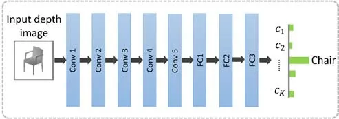
Fig.4 Architecture of our shape classif ier,which is borrowed from Alex Net[25].It takes depth images as input,and outputs classif ication results.

At inference time,given an object,a depth image is generated using a ray casting algorithm with a random initial view from our selected 50 views.The generated depth image is then passed into our attentional model.The latter f irstly extracts features from the depth image,which are then used both for object classif ication(SC)and next-best-view prediction(3D-STN).Our 3D-STN automatically regresses the update to the current view.Given the current view and the view update,our camera moves to the next-best-view,and generates a new depth image.RNN hidden layers help to aggregate current depth image features with those from the past views.This is repeated until termination conditions are met.We set two termination conditions for inference:(i)the classif ication uncertainty,measured by the Shannon entropy of the classif ication probability,is less than a threshold(0.1),or(ii)the maximum number(10)of time steps has been reached.

4 Experimental setup

4.1 3D shap e datasets

Our method has been evaluated using three large-scale 3D shape datasets:ModelNet10[27],ModelNet40[3],and ShapeNet Core55[28]. ModelNet10 and ModelNet40 are two subsets of the Princeton ModelNet which contains 127,915 3D shapes categorized into 660 classes.ModelNet10 contains 10 categories with a total of 4899 3D shapes;these shapes are split into a training set and a test set.The training set contains 3991 shapes,while the test set contains 908 shapes.ModelNet40 contains 12,311 3D shapes in 40 classes;they are also split into a training set(9843 3D shapes)and a test set(2468 3D shapes).ShapeNetCore55 is a richly-annotated,large-scale dataset of 3D shapes,which has 55 common object categories with about 51,300 unique 3D shapes.For ShapeNetCore55,we split all shapes of each class into training(80%)and testing(20%)subsets.

Before training,the center of each 3D shape is placed at theorigin of thespherical coordinatesystem,and the shape is scaled to the range[−0.5,0.5].The radius of the spherical coordinate system is set to 1.During training,a 3D shape needs to be rendered into a 227×227 depth image from any given viewpoint,using the ray casting algorithm(implemented in parallel on the GPU).All depth values are normalized to[0,255].If a ray does not hit the shape,the related depth value is set to 255.

4.2 Parameters of subnetworks

We use the ReLU activation functions for all hidden layers,f(x)=max(0,x),for fast training. The shape classif ier has the AlexNet architecture[25]which contains 5 convolutional layers and 3 fully connected layers followed by a soft-max layer(see Fig.4).The same parameter settings as used in the original paper are used for the various layers.The 3D-STN contains 5 convolutional layers(shared with the shape classif ier)and 2 fully connected layers.In summary,there are about 62M parameters in total being optimized when training the 3D-STN,RNN,and SC.The maximum number of views for each view sequence is 10,the learning rate of pretraining the SC is set to 0.01,and the learning rate of joint training the 3D-STN,SC,and RNN is set to 0.001.

5 Results and evaluation

5.1 Hidden layer size

The size of the hidden layer is clearly an important hyper-parameter that af fects the performance of recurrent neural networks.In this experiment,we evaluated the ef fect of hidden layer size.We carried out object recognition experiments on ModelNet40 to determine accuracy.Five views were used for each sequence,and the radius(R)remained 1.

The candidate sizes of the hidden layer were 64,128,256,512,and 1024.Results are shown in Table 1,and show that our recurrent neural network achieves best performance with a hidden layer size of 256.All the following experiments were conducted with a f ixed hidden layer size of 256.

Table 1 Ef fect of hidden layer size on accuracy using ModelNet40

5.2 Rad ius

We use a f ixed radius of spherical coordinate system in our experiments.However,the radius has a big impact on the recognition performance.If the radius is too large,the 3D shape will be very small in projection on the depth image plane.The aim of this experiment is to f ind the best radius for our task.

All 3D shapes were scaled to the range[−0.5,0.5].We conducted a comparison using dif ferent radii:0.5,1.0,1.5,2.0,and 2.5 using ModelNet40 and 5 views.Results are shown in Table 2.Best results are obtained with a radius of 1.0,under the condition that we scale our 3D shape to a range of[−0.5,0.5].Results show that camera should neither be too far nor too near to the 3D shape.If the camera is too far from the 3D shape,accuracy will drop dramatically.However,if the camera is too near to the3D shape,theshapeprojection in thedepth image will be clipped,decreasing the recognition accuracy.Moreover,if the projection of the 3D shape spans the full depth image,some details of the shape border will be lost during the convolution operation.

5.3 Next best view

We tackle the next-best-view(NBV)problem as seeking single camera views in order to improve accuracy of 3D shape recognition.In this setting,f inding the NBV can be seen as an incremental approach to a sensing strategy for multi-view active object recognition,which always tries to achieve the highest possible accuracy with the smallest number of views.But,with partial observation of a 3D shape,it is impossible to acquire the globally optimal NBV,so we use two criteria for evaluating NBV estimation:recognition accuracy and information gain.

To evaluate the performance of NBV estimation,we compare our attentional method against four alternatives,including a baseline method and three state-of-the-art methods.The baseline method Rand selects the next view randomly.The state-of-theart NBV techniques used for comparison include 3DShapeNets[3],MV-RNN[5],and the active recognition method based on Pairwise learning[29].We trained our model on the training set from

Table 2 Ef fect of radius on accuracy using ModelNet40

ModelNet40 with the task of classif ication over its 40 classes,and tested on the ModelNet40 test set.For a fair comparison of the quality of the determined NBVs,all methods were evaluated only with depth images.We let each method predict their own NBV sequences,and uniformly used a pre-trained multiview CNN shape classif ier(MV-CNN)[30]for shape classif ication.Figure 5 plots the recognition rate versus the number of predicted NBVs.Our method achieves the fastest accuracy increase.

To further evaluate the computed NBVs,we plot in Fig.6 theinformation gain for dif ferent NBV methods.The information gain is measured by the decrease of Shannon entropy of the classif ication probability distributions:

Fig.6 Information gain for views selected by f ive methods(Rand,3DShapeNets[3],MV-RNN[5],Pairwise[29],and ours).

5.4 3D shap e recognition

To evaluate recognition performance,we carried out a comparison experiment using three datasets:ModelNet10,ModelNet40,and ShapeNetCore55.We compared our method against recent competing methods: 3DShapeNets[3],MV-RNN[5],and Pairwise learning[29].For a fair comparison,all methods were evaluated only with depth images.For 3DShapeNets and Pairwise learning,we selected the next view along the sequence by following a straight path around the viewing sphere from the beginning to the end of the sequence[29].

Table 3 shows the recognition results for a random initial view from our selected 50 views.Our method achieves the best results.We note that 3DShapeNets[3],MV-RNN[5],and our methods are depth-based,while Pairwise learning[29]uses both grayscale and depth images.In our experiment,however,we only use depth images for Pairwise learning to ensure a fair comparison.

We also note that VERAM[6]achieves a recognition accuracy of 92.1%on ModelNet40 with 9 views of gray images.They align all shapes and render 144 gray images for each shape with a Phong ref lection model.Reinforcement learning is adapted to solve the problem that gradients from observation subnetworks cannot be back propagated to recurrent subnetworks. They integrate view conf idence and view location constraints into the reward function.Moreover,three strategies(sign,clamp,and ELU)are deployed to enhance gradients.For the RNN,they deploy long short-term memory(LSTM)units.For a fair comparison,we tested with three experimental settings of VERAM.Firstly,we changed 144 viewpoints to 50 viewpoints.Secondly,we used our ray casting method to generate depth images instead of Phong gray images.Thirdly,we modif ied the LSTM of RNN to use linear mapping to keep the same setting as our method.Both VERAM and our method use AlexNet and thesame radius.We found that this modif ied VERAM gives a recognition accuracy of 88.7%for ModelNet40 with 9 views,which is inferior to our method(89.8%).

5.5 Timings

Table 4 lists the training and testing time for our method on both ModelNet10 and ModelNet40 datasets.Since the shape classif ier is pre-trained outside the joint training networks(3D-STN,RNN,and SC),we report its pre-training time separately.Table 5 compares the training time of three methods:3DShapeNets,MV-RNN,and ours,for ModelNet40.The training of 3DShapeNets involves learning the generative model with CDBN.MVRNN is trained with reinforcement learning.The comparison shows the improved training ef ficiency of our model compared to the two alternatives.All timings were obtained on a workstation with an Intel Xeon E5-2670@2.30GHz×24 with 64GB RAM and an Nvidia Titan Xp graphics card with 12GB memory.

5.6 Visualization

To visually investigate the behavior of our model,we visualize in Fig.7 view sequences produced by Pairwise learning[29]and our method.Theresults demonstrate that our method can correctly recognize the objects with plausibly planned views.We note that the regressed view sequences tend to have better coverage of shapes giving higher recognition rates than Pairwise learning.In our method,we start training our model from separate 50 initial views,which means we can start from dif ferent initial views when testing.More results of our method are shown in Fig.8.All input objects are from the test set of ModelNet40.

Table 3 Recognition accuracy for four methods and three datasets

Table 4 Training and testing time for our method

Tab le 5 Training and testing time for 3DShapeNets,MV-RNN,and our method

Fig.7 View sequences produced by Pairwise learning[29]and our method for objects from ModelNet40.

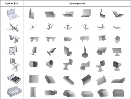
Fig.8 Visualization of the active recognition process by showing the NBV sequence with depth images for input objects from ModelNet40.

6 Conclusions

6.1 Summary

We have proposed a 3D attentional formulation for the active object recognition problem.This was mainly motivated by the resemblance of mechanisms of human attention and active perception[31],and the signif icant progress made in utilizing attentional models to address complicated vision tasks such as image captioning[8].In developing such a model,we utilized RNNs for learning and storing the internal representation of the object being observed,CNNsfor performing depth-based recognition,and STNs for selecting the next-best-views.The carefully designed 3D STN makes the whole network dif ferentiable and hence easy to train.Experiments on well-known datasets demonstrate the ef ficiency and robustness of our active recognition model.

6.2 Limitations

A drawback of learning a policy of fline is that physical restrictions during testing are hard to incorporate and when the environment is changed,the computed policy may no longer be useful.This problem can be alleviated by learning from a large amount of training data using a high capacity learning model such as deep neural networks,as we do.Our method does not handle mutual occlusion between objects which is a frequent case in cluttered scenes.One possible solution is to train the recognition network using depth images with synthetic occlusion.

6.3 Future work

In future,we would like to investigate a principled solution for handling object occlusion in real indoor scenes,e.g.,by using an STN to help localize those shape parts which are both visible and discriminative,in a similar spirit to Ref.[32].Another interesting direction is to study multi-agent attention in achieving cooperative vision tasks,such as multirobot scene reconstruction and understanding.It would be particularly interesting to study the shared and distinct attentional patterns of heterogeneous robots such as mobile robots and drones.

Acknowledgements

We thank the anonymous reviewers for their valuable comments. This work was supported,in part,by National Natural Science Foundation of China(Nos.61572507,61622212,and 61532003).Min Liu is supported by the China Scholarship Council.