A Deep Collocation Method for the Bending Analysis of Kirchhoff Plate

Hongwei Guo,Xiaoying Zhuang, and Timon Rabczuk

Abstract:In this paper,a deep collocation method (DCM) for thin plate bending problems is proposed.This method takes advantage of computational graphs and backpropagation algorithms involved in deep learning.Besides,the proposed DCM is based on a feedforward deep neural network (DNN) and differs from most previous applications of deep learning for mechanical problems.First,batches of randomly distributed collocation points are initially generated inside the domain and along the boundaries.A loss function is built with the aim that the governing partial differential equations (PDEs) of Kirchhoff plate bending problems,and the boundary/initial conditions are minimised at those collocation points.A combination of optimizers is adopted in the backpropagation process to minimize the loss function so as to obtain the optimal hyperparameters.In Kirchhoff plate bending problems,the C 1 continuity requirement poses significant difficulties in traditional mesh-based methods.This can be solved by the proposed DCM,which uses a deep neural network to approximate the continuous transversal deflection,and is proved to be suitable to the bending analysis of Kirchhoff plate of various geometries.

Keywords:Deep learning,collocation method,Kirchhoff plate,higher-order PDEs.

1 Introduction

Thin plates are widely employed as basic structural components in engineering fields[Ventsel and Krauthammer (2001)],which combines light weight,efficient load-carrying capacity,economy with technological effectiveness.Their mechanical behaviours have long been studied by various methods such as finite element method [Bathe (2006);Hughes (2012); Zhuang,Huang,Zhu et al.(2013)],boundary element method[Katsikadelis (2016); Brebbia and Walker (2016)],meshfree method [Nguyen,Rabczuk,Bordas et al.(2008)],isogeometric analysis [Nguyen,Anitescu,Bordas et al.(2015)],and numerical manifold method [Zheng,Liu and Ge (2013); Guo and Zheng (2018); Guo,Zheng and Zhuang (2019)].The Kirchhoff bending problem is a classical fourth-order problem,its mechanical behaviour is described by fourth-order partial differential equation which poses difficulties to construct a shape function to be globallyC1continuous but piecewiseC2continuous,namely,H2regular,for those mesh-based numerical method.However,according to the universal approximation theorem,see Cybenko [Cybenko (1989)] and Hornic [Hornik (1991)],any continuous function can be approximated arbitrarily well by a feedforward neural network,even with a single hidden layer,which offers a new possibility of analyzing Kirchhoff plate bending problems.

Deep learning was first brought up as a new branch of machine learning in the realm of artificial intelligence in 2006,which uses deep neural networks to learn features of data with high-level of abstractions [LeCun,Bengio and Hinton (2015)].The deep neural networks adopt artificial neural network architectures with various hidden layers,which exponentially reduce the computational cost and amount of training data in some applications [Al-Aradi,Correia,Naiff et al.(2018a)].The major two desirable traits of deep learning lie in the nonlinear processing in multiple hidden layers in supervised or unsupervised learning [Vargas,Mosavi and Ruiz (2018)].Several types of deep neural networks such as convolutional neural networks (CNN) and recurrent/recursive neural networks (RNN) [Patterson and Gibson (2017)] have been created,which further boost the application of deep learning in image processing [Yang,MacEachren,Mitra et al.(2018)],object detection [Zhao,Zheng,Xu et al.(2019)],speech recognition [Nassif,Shahin,Attili et al.(2019)] and many other domains including genomics [Yue and Wang(2018)] and even finance [Fischer and Krauss (2018)].

As a matter of fact,artificial neural networks (ANN) which are main tools in deep learning have been around since the 1940’s [McCulloch and Pitts (1943)] but have not performed well until recently.They only became a major part of machine learning in the past few decades due to strides in computing techniques and explosive growth in date collection and availability,especially the arrival of backpropagation technique and advance in deep neural networks.However,based on the function approximation capabilities of feed forward neural networks,ANN were adopted to solve partial differential equations (PDEs) [Lagaris,Likas and Fotiadis (1998); Lagaris,Likas and Papageorgiou (2000); McFall and Mahan (2009)],which results in a solution that can be described by a closed analytical form.Due to vanishing gradients,neural networks with many hidden layers require a long time for training.However,pretraining,which sets the initial values of connection weights and biases,with back propagation algorithm are now proposed to solve this problem more efficiently.More recently,with improved theory incorporating unsupervised pre-training,stacks of auto-encoder variants,and deep belief nets,deep learning has become a central and popular branch in research and applications.Some researchers employed deep learning for the solution of PDEs.Mills et al.deployed a deep conventional neural network to solve schrö dinger equation,which directly learned the mapping between potential and energy [Mills (2017)].E et al.applied deep learning-based numerical methods for high-dimensional parabolic PDEs and back-forward stochastic differential equations,which was proven to be efficient and accurate for 100-dimensional nonlinear PDEs [E,Han and Jentzen (2017); Han,Jentzen,and E (2018)].Also,E and Yu proposed a Deep Ritz method for solving variational problems arising from partial differential equations [E and Yu (2018)].Raissi et al.applied the probabilistic machine learning in solving linear and nonlinear differential equations using Gaussian Processes and later introduced a data-driven Numerical Gaussian Processes to solve time-dependent and nonlinear PDEs,which circumvented the need for spatial discretization [Raissi,Perdikaris and Karniadakis (2017a); Raissi and Karniadakis (2018); Raissi,Perdikaris and Karniadakis (2018)].Later,Raissi et al.[Raissi,Perdikaris and Karniadakis (2017b,2017c); Raissi,Perdikaris and Karniadakis(2019)] introduced a physical informed neural networks for supervised learning of nonlinear partial differential equations from Burger’s equations to Navier-Stokes equations.Two distinct models were tailored for spatio-temporal datasets:continuous time and discrete time models.They also applied a deep neural networks in solving coupled forward-backward stochastic differential equations and their corresponding high-dimensional PDEs [Raissi (2018)].Beck et al.[Beck,Becker,Grohs et al.(2018);Beck,E and Jentzen (2019)] studied the deep learning in solving stochastic differential equations and Kolmogorov equations.Nabian and Meidani studied the presentation of high-dimensional random partial differential equations with a feed-forward fully-connected deep neural networks [Nabian and Meidani (2018a,2018b)].Based on the physics informed deep neural networks,Tartakovsky et al.studied the estimation of parameters and unknown physics in PDE models [Tartakovsky,Marrero,Perdikaris et al.(2018)].Qin et al.applied the deep residual network and observation data to approximate unknown governing differential equations [Qin,Wu and Xiu (2018)].Sirignano et al.[Sirignano and Spiliopoulos (2018)] gave a theoretic motivation of using deep neural networks as PDE approximators,which converged as the number of hidden layers tend to infinity.Based on this,a deep Galerkin method was tested to solve PDEs including high-dimensional ones.Berg et al.[Berg and Nyströ m (2018)] proposed a unified deep neural network approach to approximate solutions to PDEs and then used deep learning to discover PDEs hidden in complex data sets from measurement data [Berg and Nyströ m(2019)].In general,a deep feed-forward neural networks can serve as a suitable solution approximators,especially for high-dimensional PDEs with complex domains.

Some researchers studied the surrogate of FEM by deep learning,which mainly trains the deep neural networks from datasets obtained from FEM.For instance,Liang et al.[Liang,Liu,Martin et al.(2017); Liang,Liu,Martin et al.(2018)] investigated the relationship between geometric features of aorta and FEM-predicted ascending aortic aneurysm rupture risk and then a deep learning was used to estimate the stress distribution of the aorta.In this research,we will not confine deep learning application within FEM datasets.Rather,the deflection of Kirchhoff plate is first approximated with deep physical informed feedforward neural networks with hyperbolic tangent activation functions and trained by minimizing a loss function related to the governing equation of Kirchhoff bending problems and related boundary conditions hence avoiding a FEM discretization entirely.The training data for deep neural networks are obtained by randomly distributed collocation points from the physical domain of the plate.This deep collocation method can be seen as a truly mesh-free method without the need of background grids.

The paper is organized as follows:First a brief introduction of Kirchhoff plate bending strong form with typical boundary conditions is given.Then we give a short introduction to deep learning.Finally,the deep collocation method with varying hidden layers and neurons are adopted for plates with various shapes and boundary conditions to show the performance of the proposed method.

2 Kirchhoff plate bending

Based on Kirchhoff plate bending theory [Ventsel and Krauthammer (2001)],the relation between lateral deflection w(x,y) of the middle surface (z=0) and rotations about the x,y -axis can be given by:

Under the coordinate system shown in Fig.1,the displacement field in a thin plate can be expressed as:

It is obviously that the transversal deflection of the middle plane of the thin plate can be regard as the field variables of the bending problem of thin plates.The corresponding bending and twist curvatures are the generalized strains:

Therefore,the geometric equations of Kirchhoff bending can be expressed as:

with L being the differential operator defined as

Figure1:Internal force in the coordinate system

Accordingly,the bending and twisting moments,shown in Fig.1 can be obtained as:

D0is the bending rigidity,where E and ν are the Young's modulus and Poisson ratio,and h is the thickness of the thin plate.For isotropic thin plate,the constitutive equation can be expressed in Matrix form:

The shear forces can be obtained in terms of the generalized stress components:

The differential equation for the deflections for thin plate based on Kirchhoff's assumptions can be expressed by transversal deflection as:

Consequently,the Kirchhoff plate bending problems can be boiled down to a fourth order PDE problem,which pose difficulty for tradition mesh-based method in constructing a shape function to beH2regular.Moreover,the boundary conditions of Kirchhoff plate taken into consideration in this paper can be generally classified into three parts,namely,

For clamped edge boundary Γ1,are functions of arc length.

For simply supported edge boundary Γ2,is the function of arc length,too.

For free edge boundary Γ3,whereis a load exerted along this boundary.

It should be noted that n and s here refer to the normal and tangent directions along the boundaries.

3 Deep collocation method for solving Kirchhoff plate bending

3.1 Feed forward neural network

The basic architecture of a fully connected feedforward neural network is shown in Fig.2.It comprises of multiple layers:input layer,one or more hidden layers and output layer.Each layer consists of one or more nodes called neurons,shown in the Fig.2 by small coloured circles,which are the basic units of computation.For an interconnected structure,every two neurons in neighbouring layers have a connection,which is represented by a connection weight,see Fig.2,where the weight between neuron k in hidden layer l-1 and neuron j in hidden layer l is denoted by ωjlk.No connection exists among neurons in the same layer as well as in the non-neighbouring layers.Input data,defined from x1to xN,flow through this neural network via connections between neurons,starting from the input layer,through hidden layer l-1,l,to the output layer,which eventually outputs data from y1to yM.The feedforward neural network defines a mapping FNN:RN→RM.

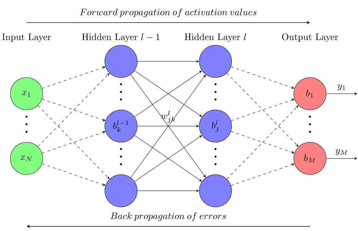
Figure2:Architecture of a fully connected feedforward back-propagation neural network

However,it should be noted that the number of neurons on each hidden layers and number of hidden layers can be arbitrarily chosen and are invariably determined through a trial and error procedure.It has also been concluded that any continuous function can be approximated with any desired precision by a feed forward neural network with even a single hidden layer [Funahashi (1989); Hornik,Stinchcombe and White (1989)].

On each neuron in the feed forward neural network,a bias is supplied including neurons in the output layer except the neurons in the input layer,which is defined by bjlfor bias of neuron j in layer l.Furthermore,the activation function is defined for an output of each neuron in order to introduce a non-linearity into the neural network and make the back-propagation possible where gradients are supplied along with an error to update weights and biases.The activation function in layer l will be denoted by σ here.There are many activation functions such as sigmoid function,hyperbolic tangent functionTanh,Rectified linear unitsRelu,to name a few.Suggestions upon their choice can be found in[Hayou,Doucet and Rousseau (2018)].Hence,for the value on each neuron in the hidden layers and output layer adds the weighted sum of values of output values from the previous layer with corresponding connection weights to basis on the neuron.An intermediate quantity for neuron j on hidden layer l is defined as

and its output is given by the activation of the above weighted input

where ykl-1is the output from the previous layer.

When Eq.(11) is applied to compute yjl,the intermediate quantity ajlis calculated'along the way'.This quantity turns out to be useful and named here as weighted input to neuron j on hidden layer l.Eq.(10) can be written in a compact matrix form,which calculates the weighted inputs for all neurons on certain layers efficiently,obtaining:

Accordingly,from Eq.(12) yl=σ(a),where activation functions are applied elementwise.A feedforward network thus defines a function f(x;θ) depending on the input data x and parametrized by θ consisting of weights and biases in each layer.The defined function provides an efficient way to approximate unknown field variables.

3.2 Backpropagation

Backpropagation (backward propagation) is an important and computationally efficient mathematical tool to compute gradients in deep learning [Nielsen (2018)].Essentially,backpropagation is based on recursively applying the chain rule and deciding which computations can be run in parallel from computational graphs.In our problem,the governing equation contains fourth order partial derivatives of field variable w(x)approximated by the deep neural networks f(x;θ).For the approximation defined by f(x;θ),in order to find the weights and biases,a loss function L(f,w) is defined to be minimized [Janocha and Czarnecki (2017)].The backpropagation algorithm for computing the gradient of this loss function L(f,w) can be defined as follows [Nielsen (2018)]:

● Input:Input dataset x1,…,xn,prepare activation y1for input layer;

● Feedforward:For each layer l=2,3,… ,L,computea n d σ(al);

● Output error:Compute the errormeasures how fast σ changes at aL;

● Backpropagation error:For each l=L-1,L-2,…,2,compute δl=

● Output:The gradient of the loss function is given by

Here,⊙ denotes the Hadamard product.

There are lists of deep learning tools to setup the training such as Pytorch or Tensorflow.The former inputs a numerical value and then computes the derivatives at this node,while the latter computers the derivatives of a symbolic variable,then stores the derivative operations into new nodes added to the graph for later use.Obviously,the latter is more advantageous in computing higher-order derivatives,which can be computed from its extended graph by running backpropagation repeatedly.Therefore,since the fourth-order derivatives of field variables is needed to be computed,the Tensorflow framework is adopted [Al-Aradi,Correia,Naiff et al.(2018b)].

3.3 Formulation of deep collocation method

The formulation of a deep collocation in solving Kirchhoff plate bending problems is introducted in this section.Collocation method is a widely used method seeking numerical solutions for ordinary,partial differential and integral equations [Atluri (2005)].It is a popular method for trajectory optimization in control theory.A set of randomly distributed points (also known as collocation points) is often deployed to represent a desired trajectory that minimizes the loss function while satisfying a set of constraints.The collocation method tends to be relatively insensitive to instabilities (such as blowing/vanishing gradients with neural networks) and is a viable way to train the deep neural networks [Agrawal].

Eqs.(8),(9)-the Kirchhoff plate bending problem-can be boiled down to the solution of a fourth order biharmonic equations with boundary constraints.Thus we first discretize the physical domain with collocation points denoted by xΩ=(x1,…,xNΩ)T.Another set of collocation points is employed to discretize the boundary conditions denoted by xΓ=(x1,…,xNΓ)T.Then the transversal deflection w is approximated with the aforementioned deep feedforward neural network wℎ(x;θ).A loss function can thus be constructed to find the optimal hyperparameters by minimizing governing equation with boundary conditions approximated by wℎ(x;θ).The mean squared error loss form is adopted here.

Substituting wℎ(xΩ;θ) into Eq.(8),we obtain

which results in a physical informed deep neural network G(xΩ;θ).

The boundary conditions illustrated in Section 2 can also be expressed by the neural network approximation wℎ(xΩ;θ) as:

On Γ1,we have

On Γ2,

where Mn(xΓ2;θ) can be obtained from Eq.(5) by combing wℎ(xΓ1;θ).

On Γ3,

where Mns(xΓ3;θ) can be obtained from Eq.(5) and Qn(xΓ3;θ) can be obtained from Eq.(7) by combing wℎ(xΓ3;θ).

It should be noted thatn,shere refer to the normal and tangent directions along the boundaries.Note the induced physical informed neural network G(x;θ),Mn(x;θ),Mns(x;θ),Qn(x;θ) share the same parameters as wℎ(x;θ).Considering the generated collocation points in domain and on boundaries,they can all be learned by minimizing the mean square error loss function:

with

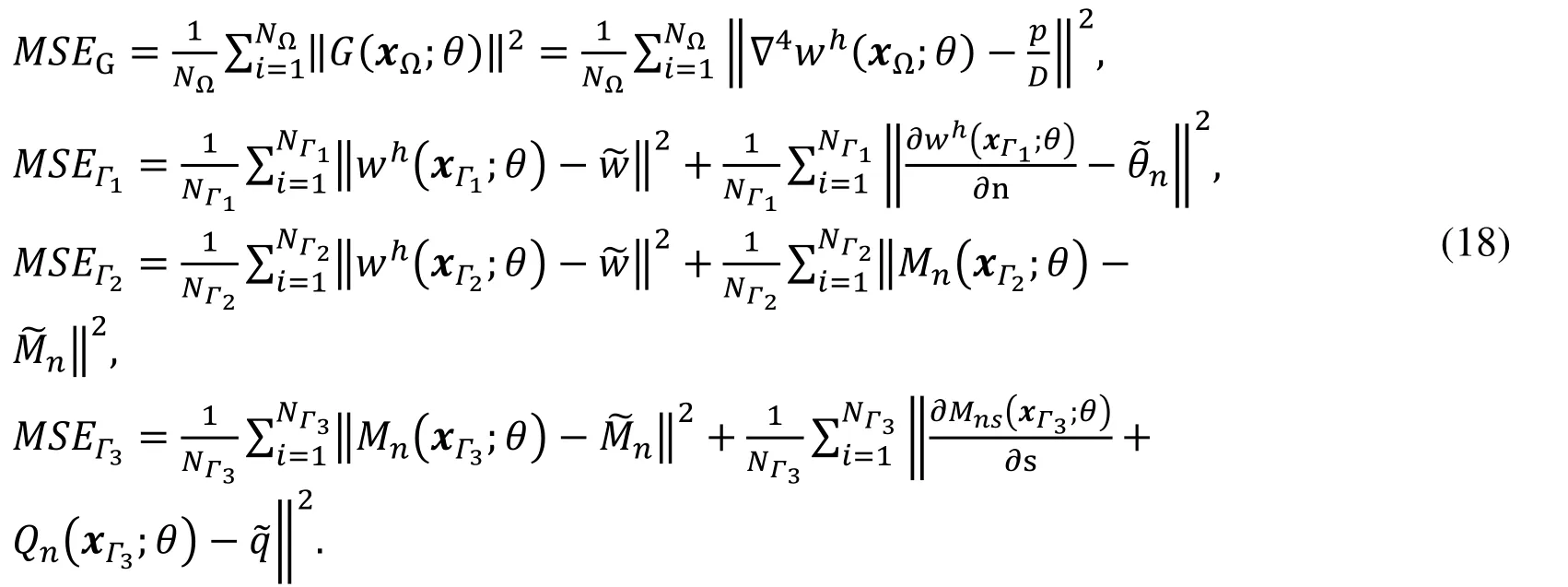
where xΩ∈ RN,θ ∈ RKare the neural network parameters.L(θ)=0,wℎ(x;θ) is then a solution to transversal deflection.Our goal is to find the a set of parameters θ that the approximated deflection wℎ(x;θ) minimizes the loss L(θ).If L(θ) is a very small value,the approximation wℎ(x;θ) is very closely satisfying governing equations and boundary conditions,namely

The solution of thin plate bending problems by deep collocation method can be reduced to an optimization problem.In the deep learning Tensorflow framework,a variety of optimizers are available.One of the most widely used optimization methods is the Adam optimization algorithm [Kingma and Ba (2015)],which is also adopted in the numerical study in this paper.The idea is to take a descent step at collocation point xiwith Adam-based learning rates αi,

and then the process in Eq.(20) is repeated until a convergence criterion is satisfied.

4 Numerical examples

In this section,several numerical examples on plate bending problems with various shapes and boundary conditions are studied.A combined optimizer suggested by Berg et al.[Berg and Nyströ m (2018)] is adopted using L-BFGS optimizer [Liu and Nocedal(1989)] first and in linear search where BFGS may fail,an Adam optimizer is then applied with a very small learning rate.For all numerical examples,predicted maximum transverse with increasing layers are studied in order to show the convergence of deep collocation method in solving the plate bending problem.

4.1 Simply-supported square plate

A simply-supported square plate under a sinusoidal distribution of transverse loading is first studied.The distributed load is given by.

Here,a,b indicate the length of the plate; D denotes the flexural stiffness of the plate depending on the plate thickness and material properties.The exact solution for this problem is given by

w represents the transverse plate deflection.For this numerical example,we first generate 1000 randomly distributed collocation points in the physical domain depicted in Fig.3.We thoroughly studied the influence of deep neural network with a varying number of hidden layer and neurons on the maximum deflection at the center of the plate,which is shown in Tab.1.The numerical results are compared with the exact solution.It is clear that the results predicted by more hidden layers are more desirable,especially for neural networks with three hidden layers.To better reflect the deflection vector in the whole physical domain,the contour plot,contour error plot of deflection for increasing hidden layers with 50 neurons are shown in Fig.5,Fig.6,Fig.7.

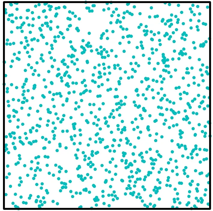
Figure3:Collocation points discretize the square domain

We employed a varying number of hidden layers from 1 to 4 and in each layer and the number of neurons varies from 20 to 60,see Tab.1.We calculated the corresponding maximum transversal deflection at the center of the square plate.The L2relative error of deflection vector at all predicted points is shown in Fig.4 for each case.Even the neural network with only one single hidden layer with 20 neurons gives very accurate results.With increasing neurons and hidden layers,the results converge to the exact solution and the results are very accurate even with a few neurons and a single hidden layer.In Fig.4,all three hidden layer types get very accurate results.Though the single layer with 20 neurons is the most accurate in all three types with 20 neurons,the magnitude of all is 10-4.As the number of hidden layers and neurons increases,the relative error flattens.

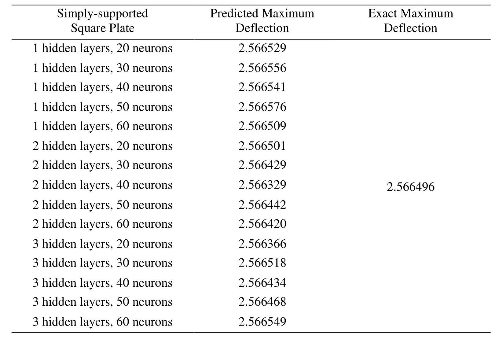
Table1:Maximum deflection predicted by deep collocation method

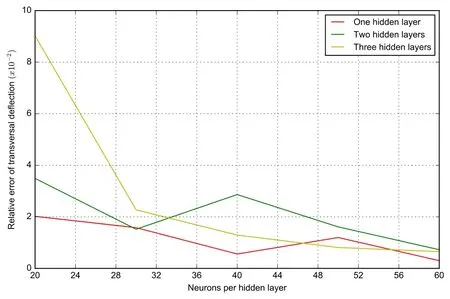
Figure4:The relative error of deflection with varying hidden layers and neurons

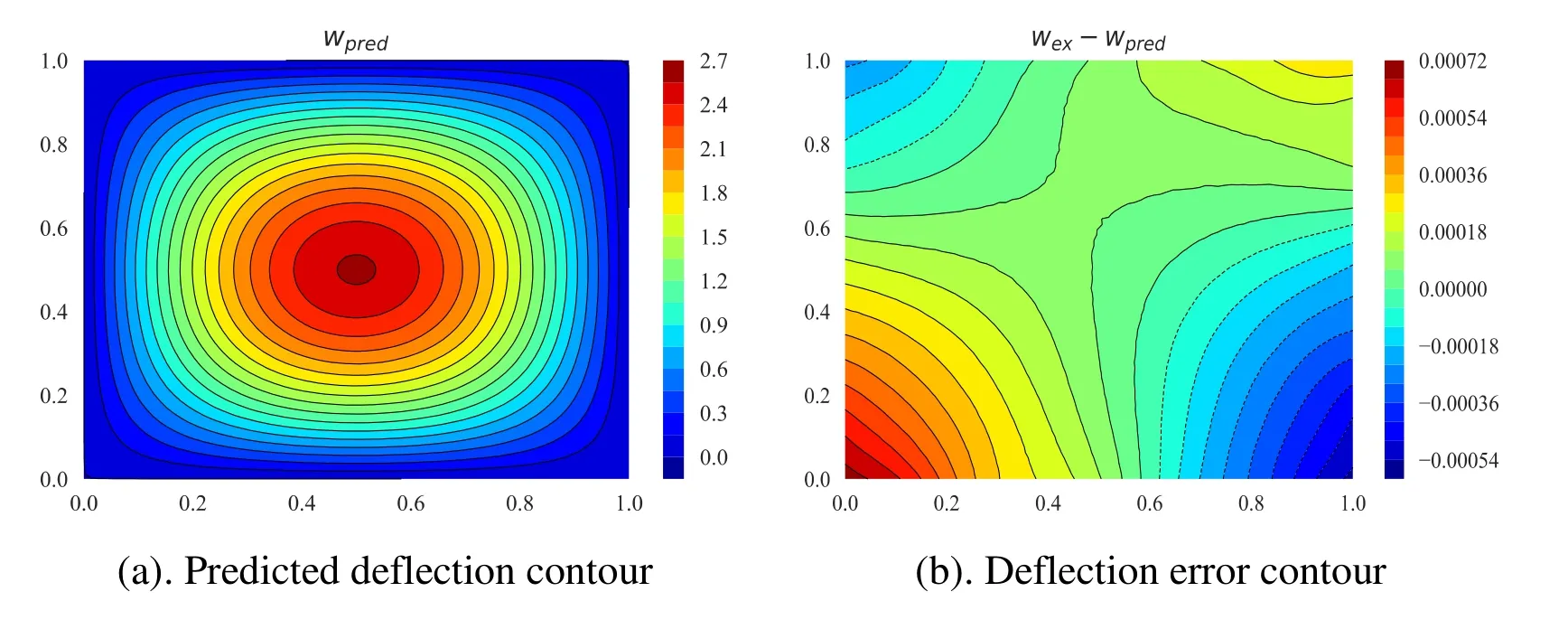
Figure6:(a) Predicted deflection contour (b) Deflection error contour (c) Predicted deflection (d) Exact deflection of the simply-supported square plate with 2 hidden layers and 50 neurons with varying hidden layers and neurons

Figure7:(a) Predicted deflection contour (b) Deflection error contour (c) Predicted deflection (d) Exact deflection of the simply-supported square plate with 3 hidden layers and 50 neurons with varying hidden layers and neurons

From Fig.5,Fig.6,Fig.7,we can observe that the deflection obtained by the deep collocation method agrees well with the exact solutions.As the hidden layer number increases,the numerical results converge to the exact solutions in the whole square plate.

The predicted plate deformation agrees well with the exact deformation.The advantages of neural networks with hidden layers are not conspicuously reflected in this numerical example,as the next numerical example shows more clearly.

4.2 Clamped square plate

Next,a clamped square plate under a uniformly distributed transverse loading is analyzed with deep collocation method.No exact solution for the deflection in the whole plate is available.Therefore,a solution obtained by the Galerkin method [Khan,Tiwari and Ali(2012)] is adopted as a comparison:

For the maximum transversal deflection at the center of an isotropic square plate,the Ritz method gives the maximum deflection at the center as[Khan, Tiwari and Ali (2012)],and Timoshenko et al.[Timoshenko and Woinowsky-Krieger(1959)] gave an exact solutionHere,D denotes the flexural stiffness of the plate and depends on the plate thickness and material properties; a,b indicate the length dimension of the plate.1000 randomly generated collocation points as in Fig.3 are used to discretize the clamped square plate.

For this clamped case,a deep feedforward neural network with increasing layers and neurons is studied in order to validate the convergence of this scheme.First,the maximum central deflection shown in Tab.2 is calculated for different number of layers and neurons and compared with aforementioned Ritz method,Galerkin method and exact solution by Timoshenko.The results of our deep collocation agree best with the exact solution.However,for neural networks with a single hidden layer,the results are less accurate,even when 60 neurons are used.As the number of neurons increases,the results are indeed more accurate for the neural network with single hidden layer.This can be observed for the other two hidden layer types.Additionally,as the number of hidden layer increases,the results are significantly more accurate than the single hidden layer neural network results.

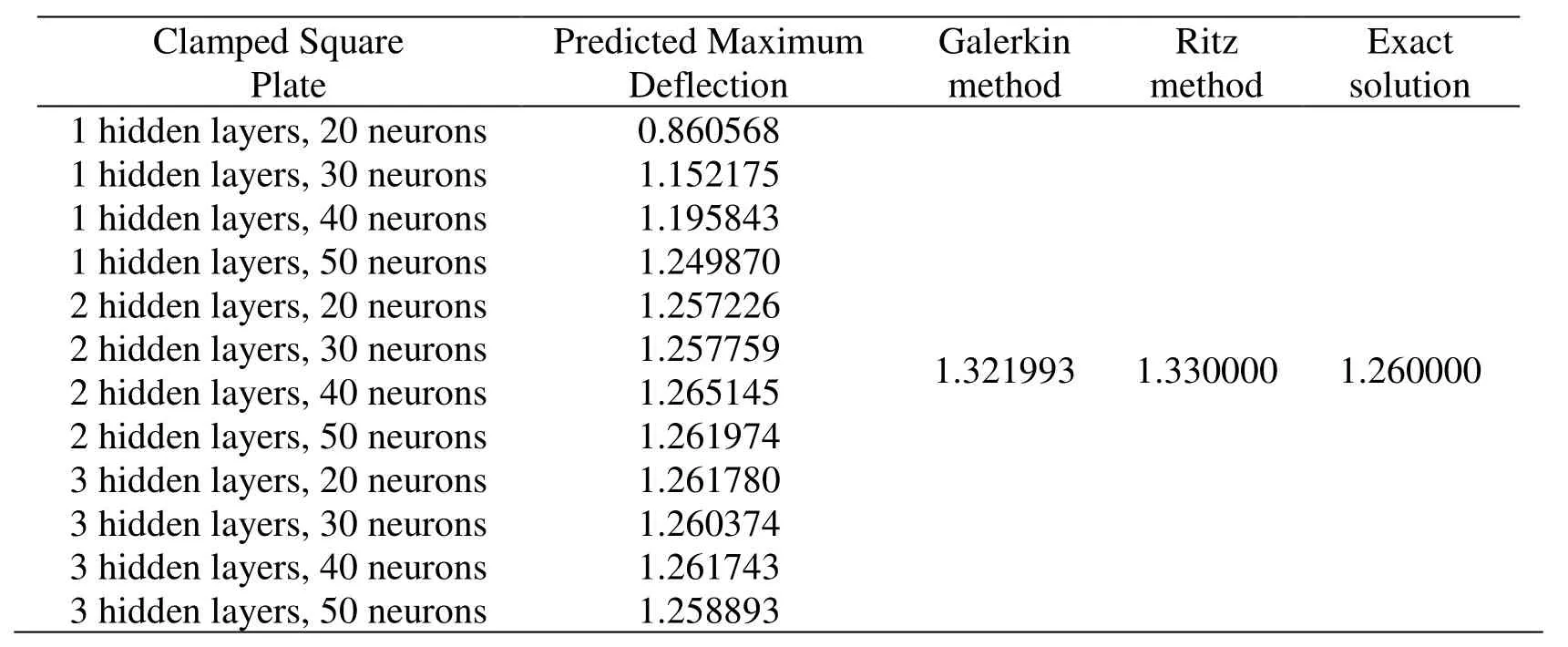
Table2:Maximum deflection predicted by deep collocation method

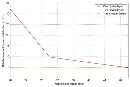
Figure8:The relative error of deflection with varying hidden layers and neurons

The relative error with the analytical solution with different hidden layers and different neurons is shown in Fig.8.The magnitude of the relative error of the deflection for this numerical example is 10-2,see also Tab.2.With increasing number of hidden layers,the two flat relative error curves coincide and converge to the exact solution.

Figure9:(a) Predicted deflection contour (b) Deflection error contour (c) Predicted deflection (d) Exact deflection of the clamped square plate with 3 hidden layers and 50 neurons with varying hidden layers and neurons

Finally,the deflection contour,relative error contour and deformed deflection of the middle surface for the deep neural network with three layers and 50 neurons is illustrated in Fig.9.

4.3 Clamped circular plate

A clamped circular plate with radius R under a uniformly distributed force is employed in the domain of the circular plate.This problem has an exact solution given by Timoshenko et al.[Timoshenko and Woinowsky-Krieger (1959)]:

D denoting the flexural stiffness of the plate.The maximum deflection at the central of the circular plate with varying hidden layers and neurons is summarized in Tab.3 and compared with the exact solution.The predicted maximum deflection becomes more accurate with increasing number of neurons and hidden layers.The relative error for deflection of clamped circular plate with increasing hidden layers and neurons is depicted in Fig.11.As hidden layer number increases,the relative error curves become flatter and converges to the exact solution.All neural networks perform well with a relative error magnitude of 10-4.

Figure10:Collocation points discretize the circular domain

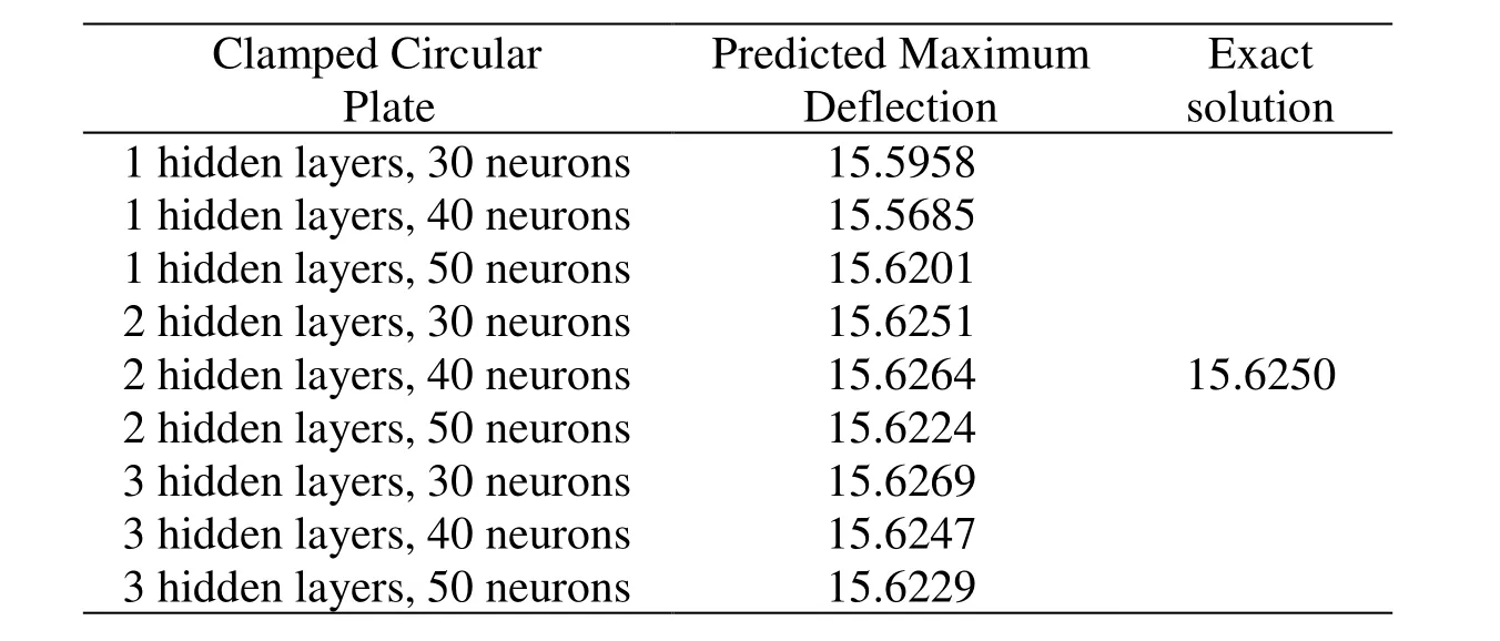
Table3:Maximum deflection predicted by deep collocation method

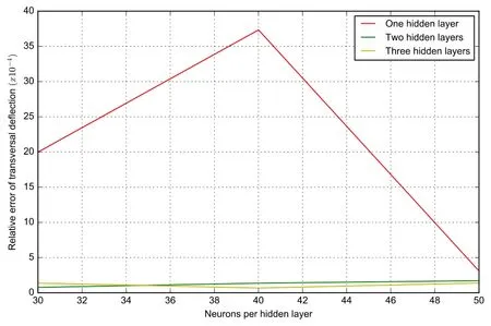
Figure11:The relative error of deflection with varying hidden layers and neurons

The deformation contour,deflection error contour,predicted and exact deformation figures are displayed in Fig.12.The deflection of this circular plate agrees well with the exact solution.

Figure12:(a) Predicted deflection contour (b) Deflection error contour (c) Predicted deflection (d) Exact deflection of the clamped circular plate with 3 hidden layers and 50 neurons with varying hidden layers and neurons

4.4 Simply-supported square plate on Winkler foundation

The last example is a simply-supported square plate resting on Winkler foundation,which assumes that the foundation's reaction p(x,y) can be described by p(x,y)=kw,k being a constant called foundation modulus.For a plate on a continuous Winkler foundation,the governing Eq.(8) can be written as:

The analytical solution for this numerical example is [Timoshenko and Woinowsky-Krieger (1959)]:

For this numerical example,the same arrangement of collocation points is depicted in Fig.3.Neural networks with different neurons and depth are applied in the calculation.Tab.3 lists the maximum deflection at the central point in all cases.Good agreement can be observed in this numerical example as well.As hidden layer and neuron number grows,the maximum deflection becomes more accurate approaching the analytical serial solution for even two hidden layers.The relative error shown in Fig.13 better depicts the advantages of deep neural network than shallow wide neural network.More hidden layers,with more neurons yield flatting of the relative error.Various contour plots are shown in Fig.14 and compared with the analytical solution.

Table4:Maximum deflection predicted by deep collocation method

Figure13:The relative error of deflection with varying hidden layers and neurons

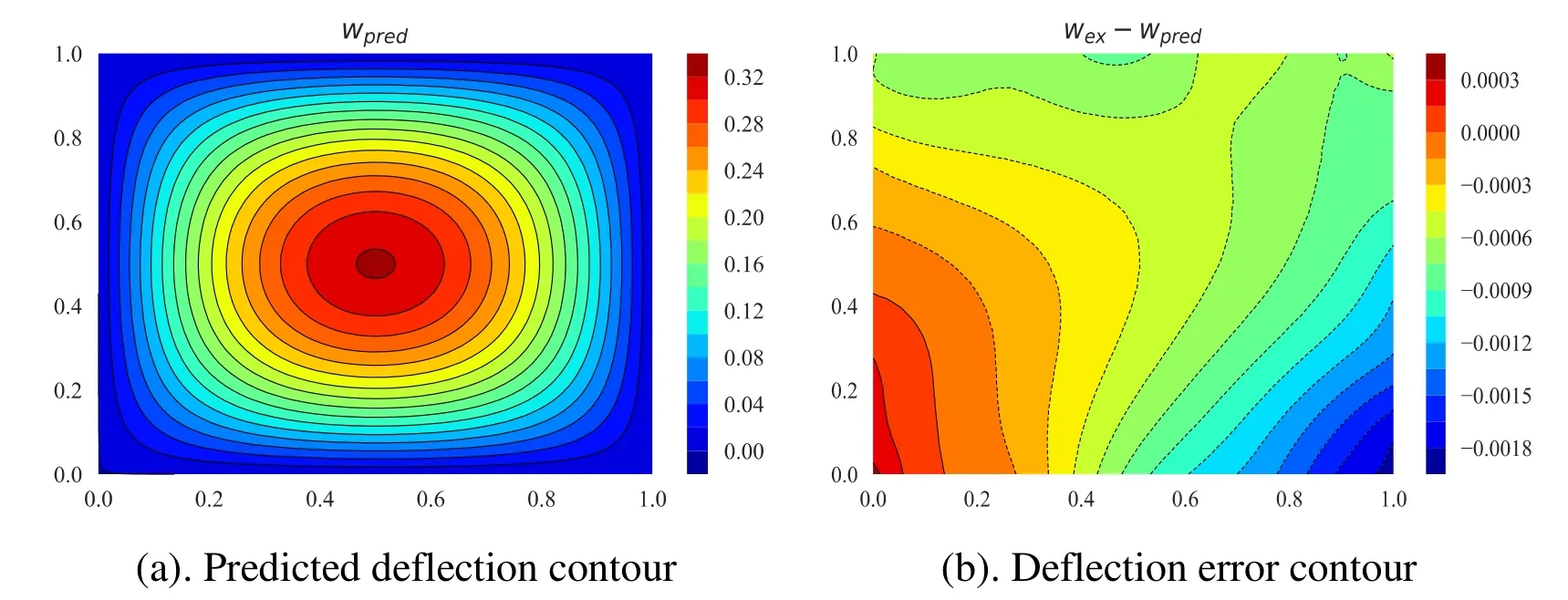
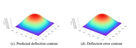
Figure12:(a) Predicted deflection contour (b) Deflection error contour (c) Predicted deflection (d) Exact deflection of the simply-supported plate on Winkler foundation with 3 hidden layers and 50 neurons with varying hidden layers and neurons

5 Conclusions

We propose a deep collocation method to study the bending analysis of Kirchhoff plates of various shapes,loads and boundary conditions.The governing equation of this problem is a fourth order partial differential equation (biharmonic equation).The proposed deep collocation method can be considered as truly "meshfree" and can be used to approximate any continuous function,which is very suitable for the analysis of thin plate bending problems.The deep collocation method is very simple in implementation,which can be further applied in a wide variety of engineering problems.

Moreover,the deep collocation method with randomly distributed collocations and deep neural networks perform very well with MSE loss function minimized by the combined L-BFGS and Adam optimizer.Accurate results are obtained even for a single layer and 20 neurons.However,as the hidden layers and neurons on each layer increase,results gain in accuracy and converge to the exact and analytical solution.Most importantly,once those deep neural networks are trained,they can be used to evaluate the solution at any desired points with minimal additional computation time.

However,there are still several issues for the deep neural network based method such as the influence of choosing other neural network types,activation functions,loss function forms,weight/bias initialization,and optimizers on the accuracy and efficiency of this deep collocation method,which will be studied in our future research.