Modelling of vehicle interaction behavior during discretionary lane-changing preparation process on freeway

Nie Jianqiang Zhang Jian Ran Bin

(1State Key Laboratory of Air Traffic Management System and Technology,The 28th Research Institute of China Electronics Technology Group Corporation, Nanjing 210007, China)(2School of Transportation, Southeast University, Nanjing 211189, China)

Abstract：In order to increase the accuracy of microscopic traffic flow simulation, two acceleration models are presented to simulate car-following behaviors of the lane-changing vehicle and following putative vehicle during the discretionary lane-changing preparation (DLCP) process, respectively. The proposed acceleration models can reflect vehicle interaction characteristics. Samples used for describing the starting point and the ending point of DLCP are extracted from a real NGSIM vehicle trajectory data set. The acceleration model for a lane-changing vehicle is supposed to be a linear acceleration model. The acceleration model for the following putative vehicle is constructed by referring to the optimal velocity model, in which optimal velocity is defined as a linear function of the velocity of putative leading vehicle. Similar calibration, a hypothesis test and parameter sensitivity analysis were conducted on the acceleration model of the lane-changing vehicle and following putative vehicle, respectively. The validation results of the two proposed models suggest that the training and testing errors are acceptable compared with similar works on calibrations for car following models. The parameter sensitivity analysis shows that the subtle observed error does not lead to severe variations of car-following behaviors of the lane-changing vehicle and following putative vehicle.

Key words：vehicle interaction behavior; discretionary lane-changing preparation process; lane-changing vehicle; following putative vehicle; optimal velocity model

The lane-changing behaviors of vehicles are complex, which play a fundamental role in the microscopic traffic flow theory. According to the intention of lane change, lane-changing behaviors are commonly categorized into two types: mandatory lane change (MLC) and discretionary lane change (DLC). The MLC describes the behavior that the vehicle must leave the current lane while the DLC is performed to improve the driving conditions. The effect of the DLC on traffic flow is scattered and global while that of the MLC is focused and local. The complete lane-changing process is composed of a lane-changing decision (LCD), lane-changing preparation (LCP) and lane-changing execution (LCE). LCD includes the following four successive decisions: Generation of the lane-changing requirement, choice of the target lane, choice of the target gap and acceptance of the target gap. The target lane is selected from the adjacent lanes and drivers seek an appropriate target gap in the target lane. According to the characteristics of driving behavior, the first two decisions have few significant effects on vehicle’s current car-following motion. After choosing a target gap, an LCP process will be executed until the target gap is acceptable for lane change. During the LCP process, especially in a congested traffic situation, the lane-changing vehicle usually has to deliberately slow down first to wait for the target gap or to speed up to squeeze into the target gap. In this process, the following putative vehicle may slow down or switch to the other lane to let the lane-changing vehicle in. Thus, a lane-changing vehicle interacts with surrounding vehicles in its current lane and target lane during the LCP process. The LCE process is the period from the time that the lane-changing vehicle accepts the target gap to the time that the lane-changing vehicle inserts itself into the target gap successfully. The LCE process occurs right after the LCP process.

LCD has been studied adequately.A comprehensive review about LCD modelling can be referred to in Refs.[1-2]. The LCD models can be classified into four groups: Rule-based models, discrete-choice models, artificial intelligence models, and incentive-based models. Rule-based models include the Gipps model[3], CORSIM model[4], SITRAS model[5], cellular automata model[6]and game theory model[7]. Discrete-choice models include Ahmed’s model[8]and Toledo et al.’s model[9]. Artificial intelligence models include the artificial neural network model[10-11]and fuzzy-logic based model[12]. Incentive-based models include MOBIL[13]and LMRS.

Recently, the research on LCE modelling has been increasing.Moridpour et al.[14]studied LCE modelling under heavy traffic conditions, and proposed the longitudinal acceleration models for both heavy vehicles and passenger cars. Papadimitriou and Tomizuka[15]proposed a polynomial model to make automated vehicles move in both longitudinal and latitudinal directions. In the manual LCE process, the lane-changing vehicle must dynamically interact with its putative leader and follower in the target lane in the longitudinal direction accompanying a lateral movement. Kou and Machemehl[16]used the angular velocity that contained the lateral motion features to build an acceleration-deceleration model for lane-changing vehicles.Wan et al.[17]introduced visual angle information to capture the vehicle interaction behavior during the LCE process. Wang et al.[18]proposed a behavioral-based general framework for the LCE model.

The drivers’ behaviors related to the LCP have been seldom paid attention to for a long time. Hidas[19]developed a new cooperative lane-changing model incorporating explicit modelling of vehicle interactions during the LCP process using intelligent agent concepts, but the model is only a concept, not yet validated by field data. Sun and Kondyli[20]quantified the vehicle interactions during the LCP process. Schakel and Knoop[21]introduced a concept of synchronized lane change which means that a potential lane-changing vehicle intends to synchronize velocity with the vehicles in the target lane. Empirical analysis based on field trajectory data was presented to support such a concept by Wan et al.[22]and Park et al.[23], but the field data was limited to the freeway merging area.

In summary,existing research about lane-changing behavior focused on LCD and LCE. Research on LCP is rare, and the research about LCP for DLC on freeways is almost ignored. Hereafter, the LCP for DLC is called discretionary lane-changing preparation (DLCP), and similarly, the LCE for DLC is called discretionary lane-changing execution (DLCE). However, the DLCP process on a freeway plays an important role in simulating and predicting the lane-changing behavior more completely and accurately. The aim of this study is to put forward two acceleration models to simulate the longitudinal driving behaviors of the lane-changing vehicle and the following putative vehicle during the DLCP process on freeway.

1 Data Description

This study used the published dataset, collected at US Highway 101(US-101) in Los Angeles, California, USA. The entire segment of US-101 is 630 m long with five freeway lanes and an auxiliary. Starting with 1, lane numbers are incremented from the left-most lane. The US-101 data was collected from 07:50 to 08:35 on June 15, 2005. The time interval for vehicle location update is 0.1 s, and each measured sample from this data set has 18 features, such as longitudinal position, lateral position, velocity, acceleration, time, vehicle class, front vehicle number, and following vehicle number. Lane 5 and 6 are excluded from the study since lane-changing behaviors in these lanes are likely affected by the on and off ramps,but not likely to be discretionary lane changes. To obtain a homogeneous model, four additional criteria are applied for the selection of the discretionary lane-changing behavior sample:

1) The lane-changing vehicles which are trucks or motorcycles are not considered.

2) The lane-changing vehicles whose interacting vehicles include trucks or motorcycles are not considered.

3) Successive lane-changing processes are not considered.

4) The failed lane-changing processes are not considered.

5) The lane-changing vehicles whose leading vehicle (in original lane) or putative leading and following vehicle (in the target lane) changes lane at the same time are not considered.

By using the above criteria, 146 discretionary lane-changing behavior samples are selected. The corresponding data set is smoothed by the locally weighted scatterplot smoother algorithm(LOWESS)[24].

2 Identification of DLCP

Fig.1 shows the layout of a lane-changing vehicle and its interacting vehicles during DLCP process, in which the lane-changing vehicle is named as a subject vehicle and marked as“SV”. Its interacting vehicles include the leading vehicle and following vehicle on the current lane as well as the putative leading vehicle and the following putative vehicle on the target lane. They are denoted as CLV, CFV, PLV and PFV, respectively, in Fig.1. The distance between SV and real CLV, CFV, PLV or PFV is beyond 135 m. If CLV (CFV, PLV or PFV) is absent within 135 m, then a corresponding virtual vehicle (CLV, CFV, PLV or PFV) is set to be located at the position where the distance to SV is 135 m. The speed of the following virtual vehicle (CFV and PFV) is set to be 0 m/s and that of leading virtual vehicle (CLV and PLV) is set to be 30 m/s. The gap between PLV and PFV is known as the target gap of subject vehicle and denoted asgT. The piece-wise line with an arrow in Fig.1 illustrates the sketch of the whole lane-changing trajectory, where the first segment represents the trajectory during the DLCP process and the second segment represents the trajectory

Fig.1 Sketch of lane-changing vehicle and its interacting vehicles’ layout during DLCP process

during the DLCE process. To systematically identify the DLCP process, the starting point and the ending point of the DLCP process should be determined.

2.1 Identification of the starting point of DLCP process

In this study, it is assumed that once SV’s DLCP behavior is initiated and PFV obtains the signal, it will start to slow down to provide a sufficient spacing with PLV for SV inserting into target lane, which is called anticipation behavior[25]. Thus, the identification of the starting point of SV’s DLCP process can be transformed into the identification of the starting point of PFV’s anticipation behavior.

So far, two ways to identify the starting point of PFV’s anticipation behavior have been presented, but both of them have their limitations in practical applications. Zheng et al.[25]used the Newell simplified car-following theory to specify the starting point of anticipation. The starting point of anticipation is identified by intersecting the theoretical time-space trajectory of the PFV with its actual trajectory before SV inserts into the target lane. The method is based on the hypothesis that the spacing-speed relationship for a given vehicle is linear before the anticipation period, which is not consistent with real data in most cases. Ghaffari et al.[26]proposed another method for the identification of the starting point of the anticipation period. In this method, the time when PFV’s acceleration reaches the maximum before SV inserts into target lane is determined as the start of anticipation behavior. In fact, this method cannot guarantee that the target gap will become more suitable for SV inserting into the target lane after the determined starting point of the anticipation period.

Thus, a simple but practical way is employed to identify the start of anticipation behavior by referring to the two methods mentioned above. In the new method, the time when the spacing between PFV and PLV starts to approximately enlarge significantly and continuously until SV gets into target lane, is taken as the start of the anticipation period. At the same time, another condition that the SV’s longitudinal position is close to the target gap should be satisfied. In this study, both the relative space between SV and PLV and the relative space between PFV and SV are constrained to range from -1.5 to 30 m. Taking the real SV with the vehicle ID of 410 for example,Fig.2 shows the identification results of the starting point of DLCP process. The perpendicular black line in Fig.2 represents the starting point of the anticipation period, which is captured accurately from an intuitive view.

2.2 Identification of ending point of DLCP process

DLCP occurs before DLCE, and the ending point of DLCP is the starting point of DLCE. Similarly, the identification of the ending point of SV’s DLCP process is transformed into the identification of the starting point of

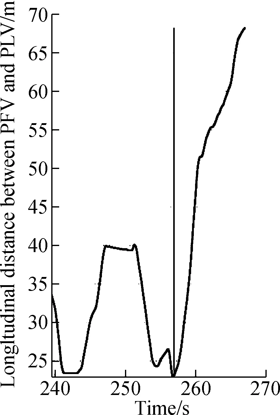
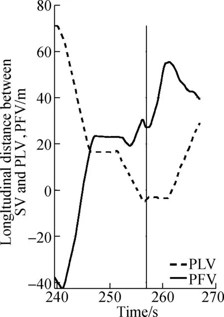
(a) (b)Fig.2 Identification of the starting point of DLCP process for SV with the vehicle ID of 410.(a) Change of longitudinal distance between PFV and PLV;(b) Change of longitudinal distance between SV and PFV, PLV

the DLCE process. The start of the lane-changing vehicle’s lateral movements toward the adjacent target lane without being interrupted is defined as the starting point of the DLCE by several researchers[14, 27]. However, this method ignores the significant change of lateral velocity when SV starts DLCE. In reality, the magnitude of lateral acceleration at this time slot often corresponds to a local maximum. Thus, in this study, when the SV moves from the original lane towards the target lane without interruption, the maximum of its lateral acceleration is denoted as the starting point of DLCE, i.e. the ending point of DLCP. Taking the real SV with the vehicle ID of 410 for example as well, the identified results of the ending point of DCLP are shown in Fig.3. The rendered black circle in Fig.3(a) and Fig.3(b)represent the identified starting point of DLCE with the traditional method and the new proposed method. In the next section, we employ the proposed method to identify the starting point of DLCE.

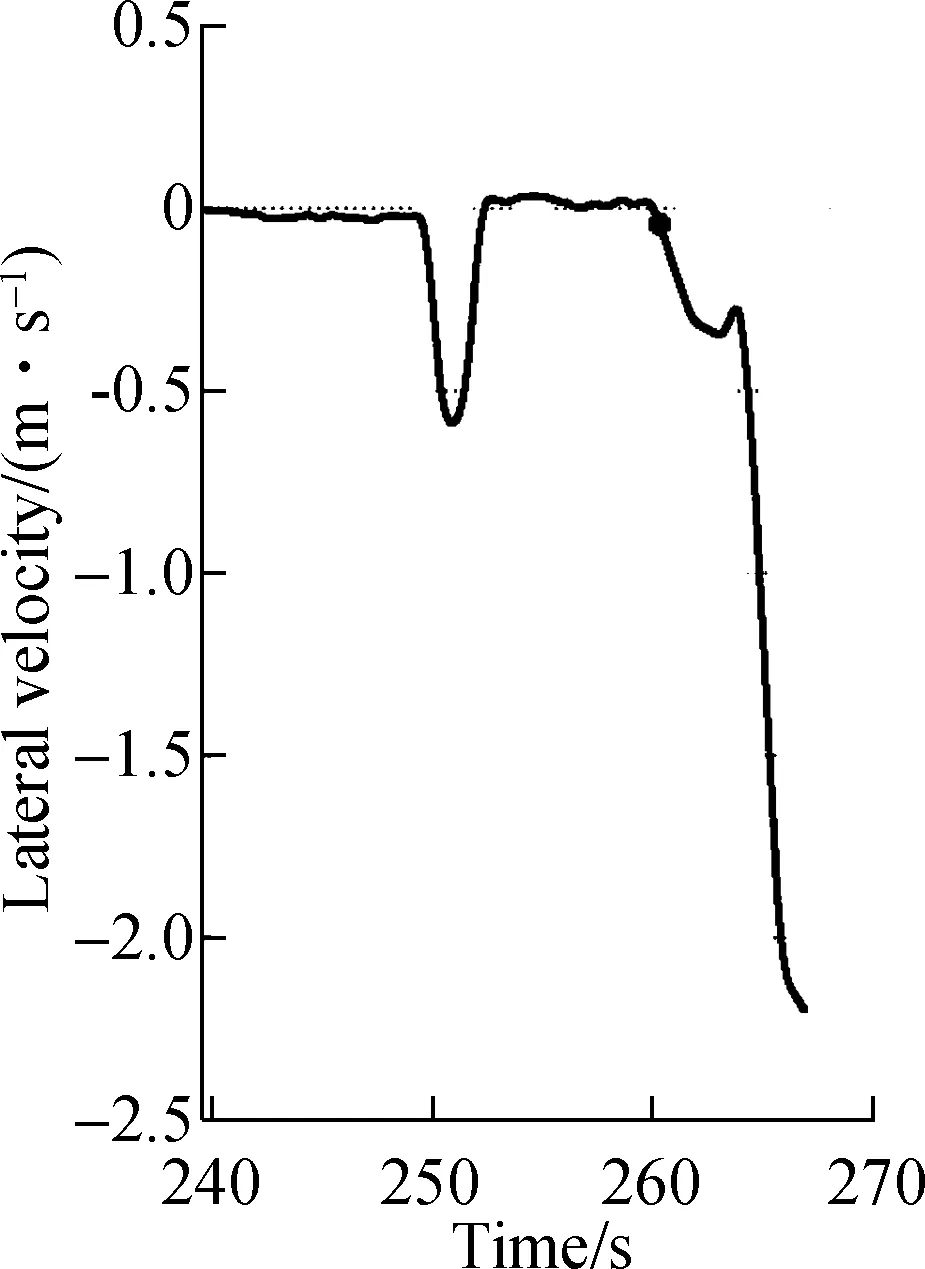
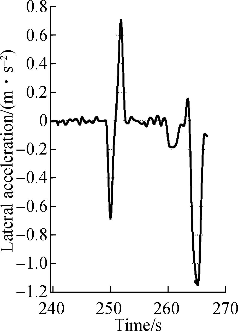
(a) (b)Fig.3 Identification of ending point of DLCP process for SV with the vehicle ID of 410.(a) Change of lateral velocity of SV;(b) Change of lateral acceleration of SV

3 Acceleration Model of Lane-Changing Vehicle during the DLCP Process

By applying the identification procedure for the trajectory of DLCP process described in Section 2 on the selected NGSIM dataset, 100 groups of samples are extracted in all. The empirical observations indicate that DLCP period persists for 4 to 8 s on average with variations across sites and lanes, which suggests that the DLCP behavior is significant and should not be ignored in modelling the lane-changing behavior. The 100 selected groups of samples are randomly divided into two equal parts (50 groups each). One is employed to calibrate the proposed model and the other is applied to validate the model performance. This section focuses on modelling the longitudinal driving behavior of lane-changing vehicles during the DLCP period.

3.1 Model formulation

For the longitudinal movement during the DLCP period, SV behaves in a similar manner as it does under the normal car following situations. The difference is that SV behaves in response to CLV, PLV, and PFV simultaneously. Thus, the longitudinal governing equation of SV during DLCP period is given as

(1)

(2)

The estimated parameters and supporting statistics indicators for the simplified model are also summarized in Tab.1.

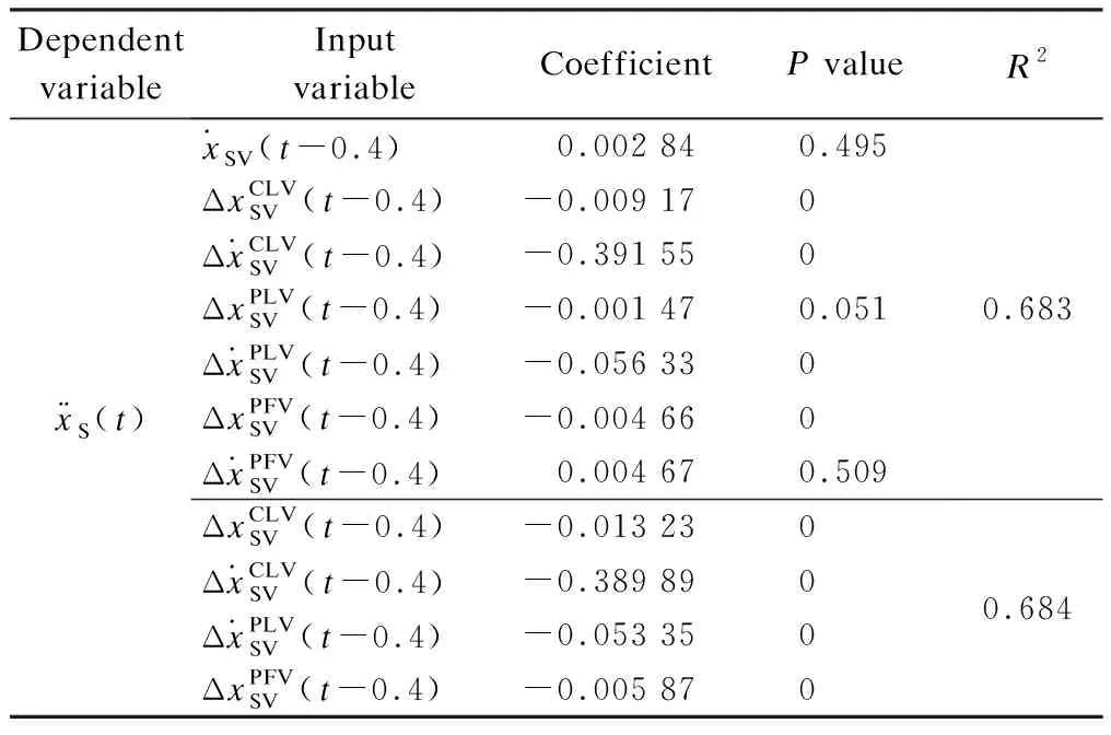
Tab.1 Summary of original and simplified modelling

3.2 Model validation

The effectiveness of the above-proposed model in replicating real longitudinal driving behavior during DLCP period is validated using the MOE (model of effectiveness) indices: MAE (mean absolute error) and RMSE (root mean square error). Their formulations are

(3)

(4)

whereMrepresents the number of all samples;mrepresents the observation instant number of sample subset; the superscript “real” and “sim” denote the values from the real dataset and the proposed model, respectively;xcan be positionp, velocityvand accelerationa.

Tab.2 exhibits the validation results of SV. Both model errors using the calibration and validation samples are within an acceptable range based on the table. Therefore, the proposed acceleration model can replicate the longitudinal driving behavior of SV during DLCP period with good performance. From Tab.2, it can be found that the MAE and RMSE ofp,vandahave great differences. This can be explained by the fact that the variation range of positions, velocity and acceleration differ greatly during the DLCP period.

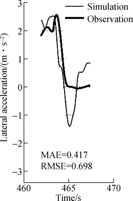
Meanwhile, we used the simplified proposed model to simulate three real DLCP trajectories selected from the aforementioned dataset. One trajectory of SV with a longitudinal speed of 7.455 m/s at the beginning of the DLCP period is selected randomly. The actual observed DLCP trajectory is used as a reference trajectory for the comparison. Fig.4 presents the simulation results of acceleration,

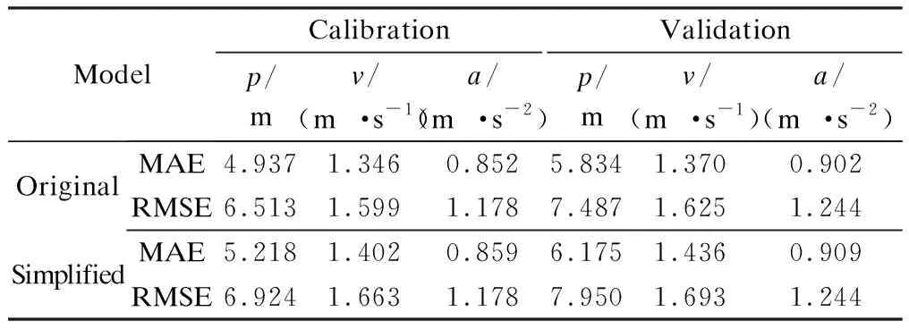
Tab.2 Summary of validation results for SV

velocity and position trajectory for the simplified proposed model. From Fig.4, errors are acceptable compared with the similar work on validations for car following models[28].

(a) (b)

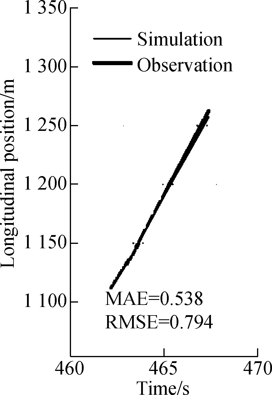
(c)Fig.4 Simulated acceleration trajectory of SV with an initial velocity of 7.455 m/s. (a) Acceleration trajectory;(b) Velocity trajectory; (c) Position trajectory

The following analysis focuses on the change of one of the MOEs, i.e. RMSE, with a subtle variation of calibrated parameters for the simplified model, since it can be seen as an indicator of the robustness of the calibration results. In Fig.5, the variations of parametersβin relation with the other three parametersγ,ωandδfor the average of all SV samples are analyzed. Here,βis restricted to the interval [-0.1, 0.1],γto [-1 1],ωto [-0.1 0.1],δto [-0.01 0.01]. Note the symmetry in each sub-figure, which is due to the linear effect of the model. The visual relationships betweenβand the other three parameters are sufficient to suggest that the calibrations forγ,ωandδare robust, exceptβ.

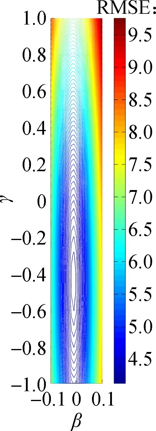
(a) (b) (c)Fig.5 Sensitivity of parameters around the found minimum RMSE of the simulated acceleration for SV. (a) Change of γ with β;(b) Change of ω with β; (c) Change of δ with β

4 Acceleration Model of following putative Vehicle during DLCP Process

In Section 3, it is mentioned that the target gap will enlarge the continuity during the DLCP period. In this section, how the target gap changes in detail will be discussed. First, the velocities of PFV versus PLV from all the observations are plotted in Fig.6. These plots reveal a obvious linear trend with a positive slope and a negative intercept. The relationship between the optimal velocity of PFV and PLV is assumed to be a linear model, which is represented by

(5)

Considering the slope of fitted straight linep1is close to 1 (see Fig.6), the slope value presumably should be 1, and Eq.(5) is simplified into

(6)

It implies that the optimal velocity of PFV relative to PLV remains stable and is equal top0during the DLCP period. Then, the next work is to estimate constant termp0more accurately again. From Eq.(6), the value ofp0is equivalent to the relative velocity with PLV of PFV. The frequency histogram for the distribution of the optimal velocity of PFV relative to PLV from all observation samples is shown in Fig.7, which is consistent with the normal distribution curve obviously. Thus, the assumption that the velocity of PFV relative to PLV obeys the normal distribution is made, and the estimation ofp0with the expectation of the fitted normal distribution, i.e.N(-6.006,37.283) is also made based on the selected samples. Therefore, Eq.(6) can be rewritten as

(7)

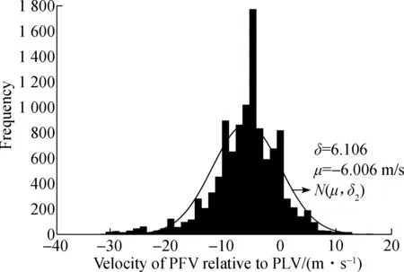
Fig.7 Distribution of velocity of PFV relative to PLV

According to Eq.(7), it can be validated that the optimal velocity of PFV is to guarantee that the target gap will be increased continuously with a stable velocity during the DLCP period.

Moreover,referring to the optimal velocity model[29]and the above-mentioned study results for lane-changing vehicle,an acceleration model is constructed to simulate the longitudinal driving behavior of PFV during the DLCP process, as follows:

(8)

(9)

By using the similar calibration method with SV’s acceleration model, the values of parametersα,β,γandTare estimated to be -0.144 14, -0.012 50, -0.101 41, and 0.4, respectively.

Tab.3 exhibits the validation results of PFV, which suggests that the proposed model has good performance in simulating the longitudinal driving behavior of PFV during the DLCP period. In Fig.8, likewise, the proposed model is used for PFV to simulate one real DLCP trajectory, with

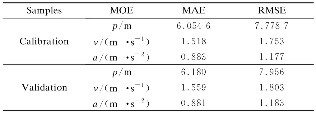
Tab.3 Summary of validation results of PFV

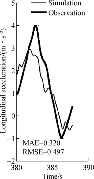
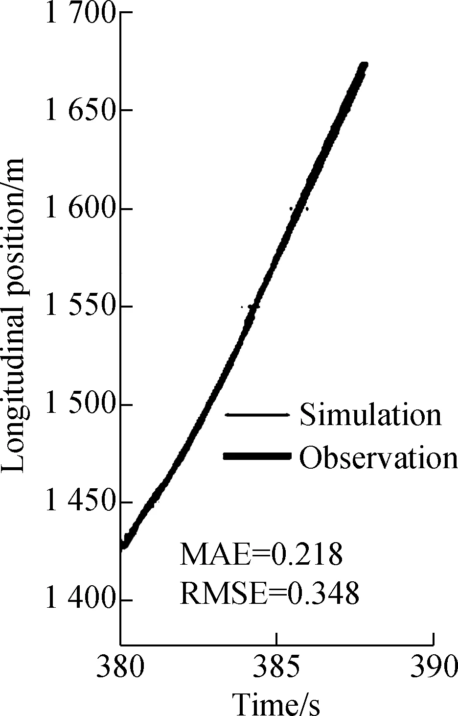
(c)Fig.8 Simulated trajectory of PFV with an initial velocity of 7.146 m/s. (a) Acceleration trajectory;(b) Velocity trajectory; (c) Position trajectory

an initial longitudinal speed of 7.146 m/s. The simulation results are acceptable as well. In Fig.9, the variation of parametersαin relation with the other two parametersβandγfor the average of all PFV samples are analyzed.αis restricted to the interval [-0.2, 0.2],βto [-0.1, 0.1],γto [-1, 1]. Here,αseems to be robust in the restricted interval, whileβandγappear to be robust only in the smaller intervals [-0.04, 0.02] and [-0.4, 0.2], respectively.

5 Conclusions

1) Two acceleration models are proposed to simulate the car-following behavior of SV and PFV during the DLCP period. Besides, two simple but practical methods are employed to identify both the starting and ending point of DLCP process, respectively. The validation results of the

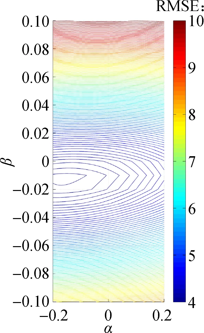
(a) (b)Fig.9 Sensitivity of parameters around the found minimum RMSE of the simulated acceleration for PFV. (a) Change of β with α;(b) Change of γ with α

linear acceleration models for SV are very close and quite acceptable compared with similar calibrations of car-following models. Moreover, the parameter sensitivity analysis suggests that the calibrated model is robust with subtle input variable observation errors.

2) The PFV acceleration model by referring to the optimal velocity model is proven to have good performance in simulating car-following behavior during the DLCP period as well. The calibrated optimal velocity function for PFV acceleration model suggests that PFV is expected to increase the target gap continuously with a stable optimal velocity relative to PLV.

3) In traditional microscopic simulation models, the DLCP process is considered to be the same as the car following phase and the longitudinal motion of lane-changing vehicle during DLCP process is simulated with regular car-following models. On the basis of identification of the starting and ending point of DLCP process from real trajectory data, the construction of the decision-making model for starting and ending the DLCP process will be our next work. The data source used in this study is limited to one dataset in NGSIM data. More datasets will be calibrated in order to validate our models in the future.