Flow induced structural vibration and sound radiation of a hydrofoil with a cavity *

Jin Tian （田锦）, Guo-qing Yuan （袁国清）, Hong-xing Hua （华宏星）

1. Institute of Vibration, Shock and Noise, Shanghai Jiao Tong University, Shanghai 200240, China

2. State Key Laboratory of Mechanical System and Vibration, Shanghai Jiao Tong University, Shanghai 200240,China

Abstract: The structural vibration and the sound radiation induced by the flow over a cavity on a hydrofoil are investigated experimentally and numerically. The large eddy simulation (LES) is adopted to calculate the flow field and the pressure fluctuation characteristics. A coupled finite element method/boundary element method approach is used to analyze the hydrofoil vibration and the structure-borne noise. The flow noise is calculated using an acoustic analogy by considering the surface pressure fluctuations as the dipole sources. A hollow hydrofoil with an orifice supported by four cylinder rods is constructed for the experiments. Modal tests are performed to obtain the natural frequencies of the hydrofoil in air and water. The vibro-acoustic experiments are carried out in the water tunnel at various free stream velocities with the orifice open and closed. A pressure transducer is used to measure the pressure fluctuations behind the downstream edge of the orifice. The triaxial accelerometers mounted on the side walls are used to measure the vibrational response of the hydrofoil. Furthermore, a hydrophone located in a box, filled with water is used to measure the sound radiation. The structure-borne noise and the flow noise are identified by their frequency properties. Reasonable agreements are observed between the numerical predictions and the experimental measurements.

Key words: Vibration, structure-borne noise, flow noise, hydrofoil, open cavity, large eddy simulation (LES)

Introduction

The flow over an open cavity attracted much interest in the past few decades, not only due to its geometrical simplicity but also due to its relevance to many practical flow problems typically found in air,ground and sea transportations. This flow is usually unsteady and the pressure fluctuations on the cavity walls might excite vibrations of the local structure,resulting in structure-borne radiated noises. The main characteristics of the cavity oscillations were first described by Rossiter[1]as a flow-acoustic resonance phenomenon, in which the oscillation frequencies were evaluated by an empirical equation.

A number of analytical models were proposed to predict the flow over cavities based on the shear layer stability theory[2]. In these models, the motion of the shear layer is associated with a transverse velocity and expressed by a sinusoidal function across the opening.The impingement of the shear layer at the downstream edge results in alternately inward and outward motions. These pulsations are fed back to the upstream edge and finally result in cavity oscillations.The vortex-sound theory was also been used to analyze the instability of the shear layer. Kook and Mongeau[3]suggested that the vortex sound was more appropriate to describe the acoustic source for the flows where the disturbance of the shear layer cannot be represented by a small wavelike motion. In their work, a similar approach was proposed and a new forward gain function was derived based on the concept of the vortex sound to model the flow excitation. Their method allowed the frequency and the relative amplitude of the cavity pressure fluctuations to be predicted for a range of flow velocities.Results show that their model predictions are in good agreement with experimental data, obtained using a rigid-wall cavity in a low-speed wind tunnel.

Experimental investigations were conducted to determine the flow characteristics of cavities with varying relative dimensions at subsonic and transonic speeds[4-6]. Crook et al.[6]carried out an experimental investigation on a supersonic flow at a freestream Mach number of 2 over a shallow open cavity,including the effects of adding streamwise serrated edges. Olsman et al.[7]carried out an experimental study of the cavity flow induced dynamic response of NACA0018 airfoil under acoustic forcing.

Cavity flow problems were also numerically investigated using the computational fluid dynamics(CFD)[8-11]. de Jong et al.[10]investigated the aeroacoustic resonance of partially covered cavities with a width much larger than their length or depth using a Lattice Boltzmann method. The predictions of the cavity flow and the flow-induced noise were made using the large eddy simulation (LES) and the FW-H acoustic analogy by Zhang et al.[11].

The aforementioned studies of the cavity flows mostly focused on the fluid oscillations, without much consideration of the vibration and the sound radiation of the cavity structure itself. However, it is of interest to examine how the cavity oscillations interact with the flexible structures, for example, in the case of an underwater vehicle, where the flow-induced vibration and the radiated sound increase the risk of being detected.

This paper presents the results of an experimental investigation of the vibration and the noise induced by the flow over a cavity on a hydrofoil in a water tunnel at different free stream velocities. Vibration data are used to identify how the pressure fluctuations excite the cavity structure and the resonance phenomenon at a specific free stream velocity. The experimental data also shed new light into the characteristics of the flow induced noise of the cavity operating in a water flow.

Numerical simulations of the flow over a hydrofoil with an open cavity are performed; results obtained numerically are compared with the experimental data.Pressure fluctuations of the cavity surface are obtained by using the unsteady three-dimensional LES. The wet modes of the hydrofoil are analyzed using a fully coupled finite element/boundary element model. The dynamic behavior and the structure-borne noise of the hydrofoil in water are obtained using a modal based vibro-acoustic response analysis. The pressure fluctuations on the hydrofoil surface are considered as the load applied on the structure. The flow noise is calculated using an acoustic analogy, in which the surface pressure fluctuations are modeled as a dipole source.

1. Experimental set-up and procedure

Experimental measurements are performed in a water tunnel at different free stream velocities to investigate the structural vibration and the sound radiation induced by the flow over the cavity on the hydrofoil. Figure 1 shows the hydrofoil geometry and the cavity area. The hydrofoil of a chord length c=382 mm is supported by four circular cylinder rods, welded to the hydrofoil side walls. The hollow hydrofoil is made of 5 mm thick steel and has a 40 mm×40 mm orifice in the middle of the upper wall. The detailed dimensions of the hydrofoil with a cavity are shown in Fig. 2.

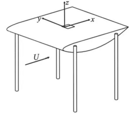
Fig. 1(a) Hydrofoil geometry

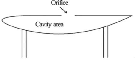
Fig. 1(b) Cavity area

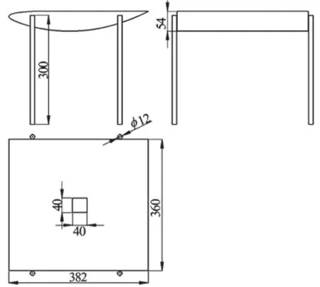
Fig. 2 Dimensions of the hydrofoil with a cavity (mm)

1.1 Modal experiments

The natural frequencies and the corresponding modal shapes of the hydrofoil in air are measured in a shaker modal test. The test set-up and the general arrangement of the instrumentation are shown in Fig.3. A Bruel & Kjaer (B & K) Type 4810 shaker is used to excite the hydrofoil and a B & K 8230 force transducer is used to measure the corresponding force applied on the hydrofoil. The structural responses are measured using 12 triaxial accelerometers (Kistler type 8763) located on the upper wall of the hydrofoil.The input force signals and the structural responses are recorded by a 32-channel LMS data acquisition system. The LMS Test. Lab is used to identify the natural frequencies and the corresponding modal shapes.

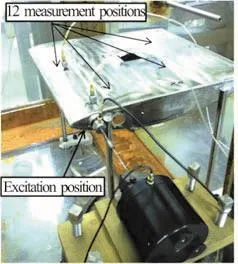
Fig. 3(a) (Color online) Experimental test set-up

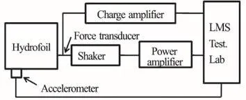
Fig. 3(b) General arrangement of the instrumentations

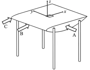
Fig. 4 The excitation positions and directions in modal tests in water

A modal test of the hydrofoil with a cavity is then carried out in water. A hammer is used to excite the hydrofoil in three positions (A, B, C) as shown in Fig.4. The excitations along y axis at point A are expected to excite the bending vibration along y. The excitations along x axis at point B are expected to excite the bending vibration along x. The excitations along x axis at point C are expected to excite the torsional vibration along z axis. One triaxial accelerometer sealed by silicon sealant is fixed on the hydrofoil surface to measure the impact response.With the procedure described in Ref. [12], a series of impact tests are performed in different positions of the hydrofoil to obtain its modal shapes and natural frequencies in water from the acceleration responses measured in the three directions (,,)x y z due to the corresponding impact.

1.2 Water tunnel vibro-acoustic experiments

The water tunnel at Shanghai Jiao Tong University is a closed-circuit, closed-jet system, having a 700 mm×700 mm square section and a length of Lw=10.6 m . A maximum water flow velocity of 5 m/s can be produced in the tunnel, corresponding to a maximum Reynolds number of 1.9×106based on the chord length c. The four rods of the hydrofoil are mounted on the floor of the water tunnel by bolt connections as shown in Fig. 5. In order to measure the sound radiation, a Plexiglas box filled with water is flush mounted to the side wall of the water tunnel.A B & K Type 8103 hydrophone is located in the middle of the Plexiglas box as shown in Fig. 5. A 5 mm diameter pressure transducer is flush mounted on the hydrofoil upper wall to measure the pressure fluctuations behind the downstream edge of the orifice.Kistler triaxial accelerometers are mounted on the two side walls of the hydrofoil and on the top of the water tunnel to measure the tunnel vibration. Table 1 lists the locations of the sensors mounted on the cavity.

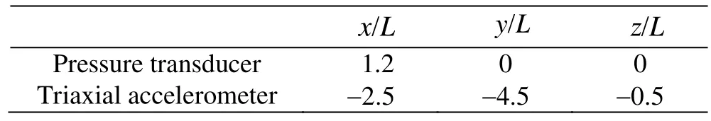
Table 1 Locations of the sensors on the hydrofoil (based on the length of the orifice L = 40 mm )

In order to obtain the experimental data with the orifice closed, a 40 mm×40 mm thin Plexiglas plate is used to seal the orifice. Experimental data of the hydrofoil obtained with the orifice open and closed are compared. In the present work, experiments are performed at various freestream velocities up to 3.5 m/s.

2. Numerical simulations

The numerical simulations are carried out in the following four steps: (1) the hydrofoil wall pressure fluctuations are computed using ANSYS-FLUENT(version 12.0), (2) the natural modes of the hydrofoil in vacuo are calculated using ANSYS, (3) the coupled modes and the vibro-acoustic responses are obtained using LMS Virtual. Lab, and (4) the flow noise is calculated using LMS Virtual. Lab. In the vibroacoustic response analysis, the pressure fluctuations obtained in step (1) are taken as the load applied on the hydrofoil structure. A flow chart diagram outlining the various steps of the numerical procedure is shown in Fig. 6. Further details of the individual steps in the numerical simulations are given in what follows.

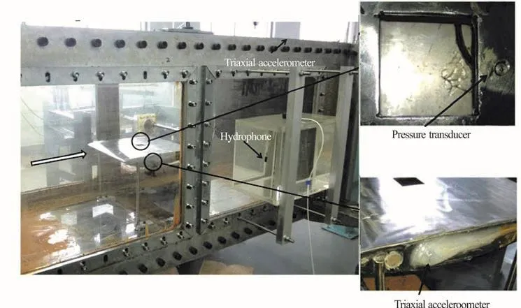
Fig. 5 (Color online) Experimental set-up in the water tunnel

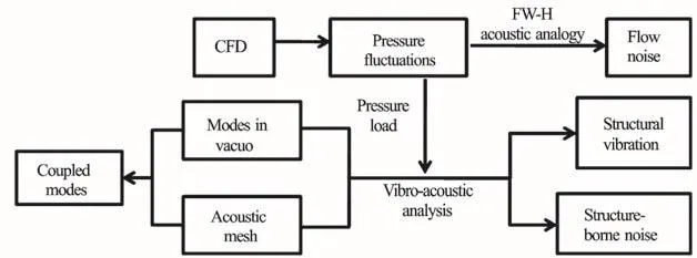
Fig. 6 Flow chart of the numerical simulations

2.1 CFD model

The LES is used to resolve the flow field around the cavity. The governing equations are obtained after filtering. The filter function G is defined and a flow variable φ is filtered as in Ref. [13]:

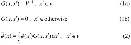
where V is the volume of a computational cell v.The governing equations for the LES are derived by filtering the time-dependent incompressible Navier-Stokes equations as

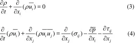
In this work, the approximate governing equations are obtained by modeling the SGS stress tensor using the Smagorinsky model. The computational domain is rectangular with the same cross-section as the water tunnel, namely 12c wide and 1.8c tall. The center of the hydrofoil is 5c from the inlet.

A model which only contains the four rods is established to calculate the unsteady force generated by the rods. The results show that the unsteady force along y axis is about 0.08 N at a free stream velocity of 3 m/s. In view of the fact that this unsteady force only makes a very small contribution to the structural response, the four rods are not included in the following CFD models.

The entire computational domain is meshed with unstructured tetrahedral cells and structured hexahedral cells. First, a grid convergence study is performed.Three types of grid density, 2.6M, 5.2M and 10.4M are studied. The model with 5.2M mixed cells are shown in Fig. 7. The unsteady force on the hydrofoil along the negative direction of z axis is selected as the monitor value for the grid convergence study. A time step of= 10-4s is selected for the calculation to ensure the convergence. A SIMPLE scheme is used for the pressure-velocity coupling. A bounded central differencing scheme is employed for the momentum equation and the second-order implicit scheme is used for the transient formulation. The velocity inlet boundary condition is specified in the flow inlet, while a pressure outlet is set for the flow outlet. A no-slip boundary condition is applied for the hydrofoil wall and the water tunnel side walls. A free stream velocity of 3 m/s is used for the grid convergence study.

Fig. 7(a) Dimensions of the computational domain

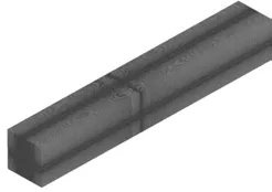
Fig. 7(b) CFD mesh of the computational domain

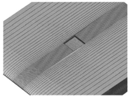
Fig. 7(c) Mesh of the cavity surface

Figure 8(a) shows the convergence history of the monitor force in cases of three grid densities. The calculation time for the unsteady simulations is 3.5 s.Figure 8(b) shows the average value of the monitor force between =3st and =3.5st . We can see that in the case of 2.6M cells we have already a converged result. By increasing the mesh resolution to 5.2M cells, one sees a decrease of the average force which is not within the defined tolerance (0.2 N) as shown in Fig. 8(b). By increasing the mesh resolution further, it can be seen that in the case of 10.4M cells,the simulation comes up with a value that is within the acceptable range. This indicates that we have reached a solution value that is independent of the mesh resolution, and in the further analysis we can use 5.2M cells, as it will give us a result within the defined tolerance.The following LES simulations are performed at the free stream velocities from 1.5 m/s-3.5 m/s. A similar CFD model is also established for the hydrofoil with the orifice closed. As shown in Fig. 9, a number of monitoring points are defined in the model to record the pressure fluctuations. The hydrofoil wall pressure fluctuations are calculated and recorded during the simulation.

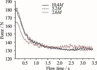
Fig. 8(a) (Color online) Convergence historyofthemonitor force of different grid densities

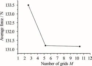
Fig. 8(b) Average value of the monitor force between =3st and =3.5st

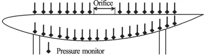
Fig. 9 Locations of the pressure monitors on xz plane, y=0

2.2 Vibro-acoustic model

The vibro-acoustic prediction is made by using a combined FEM-BEM approach. The FEM is used for the structural vibration computation and the BEM for the coupled modes and the acoustic problem by adopting an indirect formulation[14]. The fundamental governing equations of the coupled mode analyses are given in what follows. The natural frequencies of an uncoupled structure and the associated modal shapes are obtained from the following eigenvalue equation[15]

where the matricessKandsM are the stiffness and mass matrices, respectively, and u represents the displacement vector. For a fluid-loaded structure the corresponding eigenvalue equation becomes

whereaM is the added mass matrix representing the effect of the fluid loading on the structure. This added mass matrix is frequency-dependent, hence the complete coupled problem is described by

The frequency-dependent equation is approximately solved by calculating the added mass matrix at a constant frequency0ω and extracting the eigenmodes and associated eigenvalues (coupled mode eigenfrequencies) for the following approximate problem

Different coupled modal bases are obtained for different values of0ω , but in practice the difference is small, provided that0ω is within the range of the eigenfrequencies.

The FE model of the hydrofoil with a cavity is developed in the ANSYS using Solid185 and Shell63 elements. The BE model is developed in the Hypermesh. There are in total 15 000 elements in the FE model and 2 000 elements in the BE model, which are shown in Figs. 10(a), 10(b), respectively. Fixed boundary conditions are specified on the edges of the four rods. The calculated modes in vacuo and the wall pressure fluctuations are imposed as the dynamic characteristics and the load conditions for the BEM analysis, respectively. For the modes and the load conditions on the BEM surface, the modal superposition vibro-acoustic response analysis is performed to calculate the pressure and normal velocity values at all boundary nodes and field points.

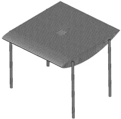
Fig.10(a) FE mesh

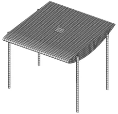
Fig.10(b) BE mesh

2.3 Flow noise model

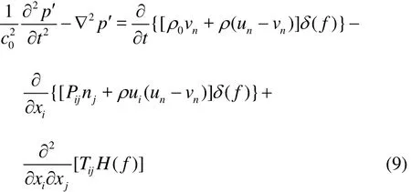
The cavity flow noise is evaluated using the Ffowcs Williams-Hawkings (FW-H) analogy. The FW-H equation simplifies the continuity and Navier-Stokes equations into the form of an inhomogeneous wave equation with two surface source terms and a volume source term as follows[16]whereiu is the fluid velocity component inix direction,nu is the fluid velocity component normal to the surface 0f= ,nv is the surface velocity component normal to the surface, ()fδ is the Dirac delta function, ()H f is the Heaviside function, p′is the sound pressure, and =0f denotes a mathematical surface introduced to the exterior flow problem ( >0)f in an unbounded space, which facilitates the use of the generalized function theory and the free-space Green function to obtain the solution. The surface ( =0)f corresponds to the source surface,and can be made coincident with a body surface or a permeable surface off the body surface.in is the unit normal vector pointing toward the exterior region.0c is the sound speed,0ρ is the far-field density andis the Lighthill stress tensor, Pijis the compressive stress tensor.

On the right hand side of the FW-H equation, the three sound source terms have clear physical meanings, which are very useful in understanding the flow noise generation. The first term corresponding to the monopole source represents the noise generated by the displacement of the fluid, the second source term corresponding to the dipole source represents the noise generated by the local pressure fluctuations, the third source term corresponding to the quadrupole source considers the nonlinear effects such as the nonlinear wave propagation, the changed local sound speed, the shock wave, the vortex and the changed turbulence. A decomposition of the sound source terms allows a simplification of the numerical calculation. The quadrupole source is ignored due to the low Mach number and the monopole source is ignored as the structural velocity is small. Only the dipole source remains the principal sound source.

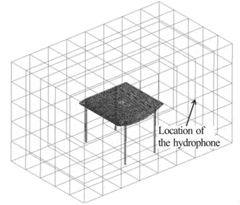
Fig.11 Acoustic and field point meshes for the flow noise calculation

In the BEM model, the wall pressure fluctuations are considered as the dipole sources. The acoustic and field point meshes for the flow noise computations are shown in Fig. 11.

3. Results and discussions

In what follows, the results of the hydrofoil modal shapes in air and in water, the pressure fluctuations over the cavity, and the dynamic response and the sound radiation of the hydrofoil obtained numerically and experimentally are discussed and compared.

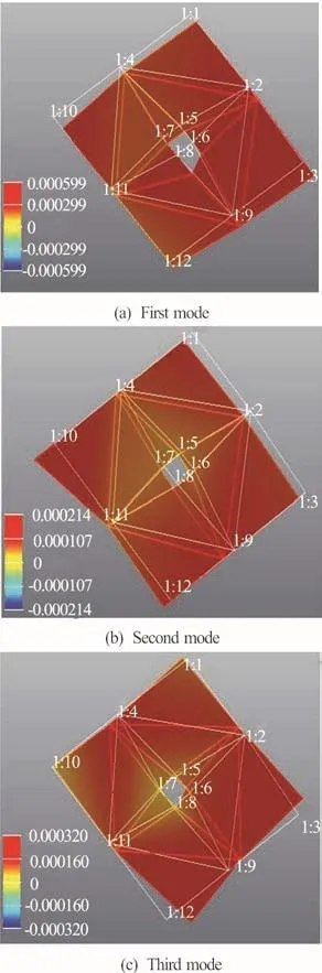
Fig.12 (Color online) Hydrofoil modal shapes in air obtained experimentally

3.1 Modal results

Due to the low flow excitation frequency, only the natural frequencies of the hydrofoil below 100 Hz are of interest. The first three modal shapes in air obtained experimentally are presented in Fig. 12,showing the undeformed (white lines) and deformed shapes (color lines). The measured resonant frequencies are 30.1 Hz, 30.3 Hz and 40.2 Hz. The first order mode is the first bending mode along the y axis, the second order mode is the first bending mode along the x axis, the third order mode is the first torsion mode around the z axis. The modal shapes obtained numerically using the FEM are shown in Fig. 13 and are in good agreement with the experimentally measured modal shapes.

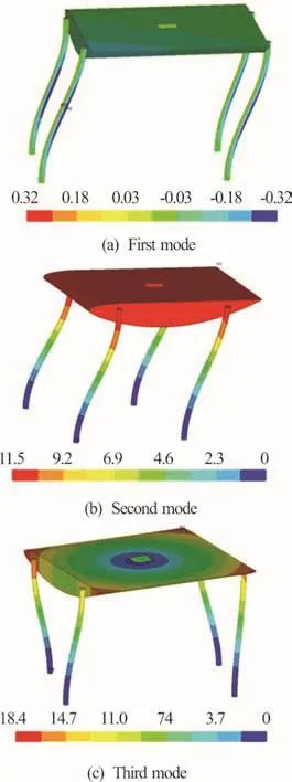
Fig.13 (Color online) Hydrofoil modal shapes in air obtained numerically

The natural frequencies of a coupled fluid-structure system are different from those of two uncoupled components. For the hydrofoil-water coupled system,the corresponding coupled modal shapes differ relatively little from the modal shapes identified in the uncoupled state[17]. Figure 14 shows the measured acceleration response by the excitations at point A in the impact tests in water.

Table 2 compares the natural frequencies of the first three modes obtained experimentally and numerically for the hydrofoil both in air and in water. The modal shapes in water remain almost unchanged and the corresponding natural frequencies are lower than their counterparts in air. The natural frequencies of the lowest order modes are more significantly affected by the fluid loading. Discrepancies between the numerical and experimental frequencies are due to the boundary conditions. In the FE simulations, fixed boundary conditions are used. In the experimental set-up, the hydrofoil is mounted using bolt connections, a combination of fixed and elastic supports.

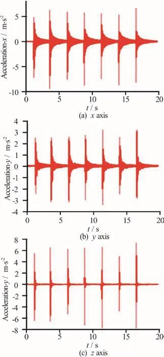
Fig.14 (Color online) Measured acceleration responses by the excitations at point A

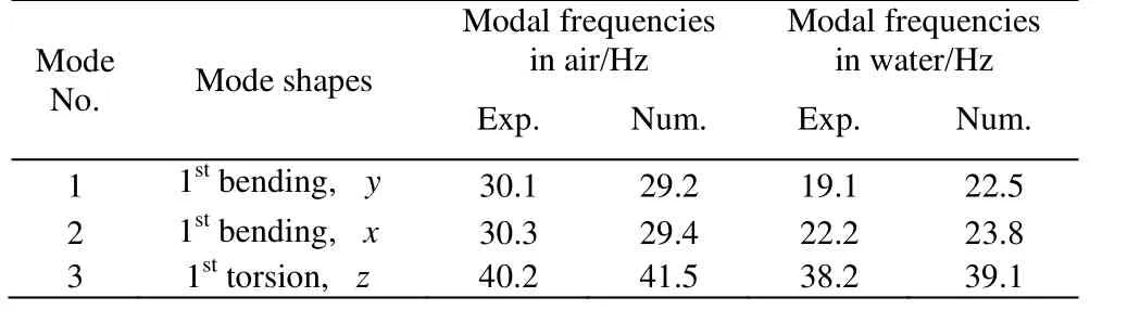
Table 2 Natural frequencies of the hydrofoil first three modes obtained experimentally and numerically, in air and in water

3.2 Flow field results

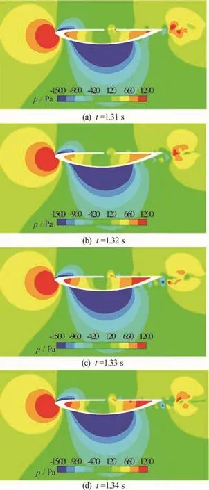
Fig.15 (Color online) Changes in pressure distribution on thecentreline plane at different time, =3.1m/s

The results from the LES simulations of the hydrofoil at different free stream velocities are presented.When the free stream velocity is equal to 3.1 m/s, thevalues in the cavity area vary from 0.8 to 1.6 and thevalues on the surface of the hydrofoil vary from 1.8 to 3.2. The centerline plane is defined as the xz plane at y = 0. Figures 15, 16 present the pressure and the Q-criterion vortex distribution at different time at a free stream velocity U =3.1m/s. It can be observed that the vortex is generated and shed from the leading edge, it then moves towards the downstream edge with the convective velocity. The impingement of the vortex at the downstream edge results in alternately inward and outward motions.These pulsations are fed back to the upstream edge and finally result in cavity oscillations. The pressure coefficient (Cp) is defined as:

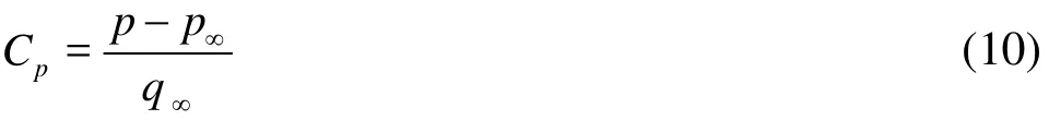
where p is the time-averaged static pressure, p∞is the free stream static pressure and q∞is the free stream dynamic pressure.

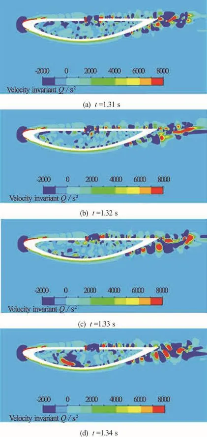
Fig.16 (Color online) Changes in vortex distribution on the centreline plane at different time, U =3.1m/s

Figure 17 presents thepC distribution on the cavity floor and the upper surface recorded by the pressure monitors described in Fig. 9. Along the first half of the cavity floor in the downstream direction,the pressure coefficient decreases until it reaches a minimum value approximately at the position / =x L 0 with a marginally negative pressure coefficient value. The pressure coefficient then increases along the second half of the cavity floor downstream,reaching a maximum value atAt the orifice areathe variation of the pressure coefficient has a profile corresponding to the transitional-closed cavity flow. The pressure fluctuating frequencies of the cavity flow can be evaluated by the empirical relationship of Rossiter as follows[1]

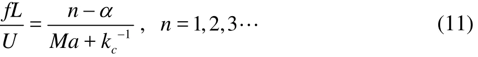
where Ma is the Mach number, α is a phase delay parameter, andck is the convection velocity coefficient.

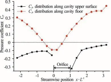
Fig.17 (Color online) Pressure coefficient distributions on the cavity floor and upper surface, U = 3.1m/ s

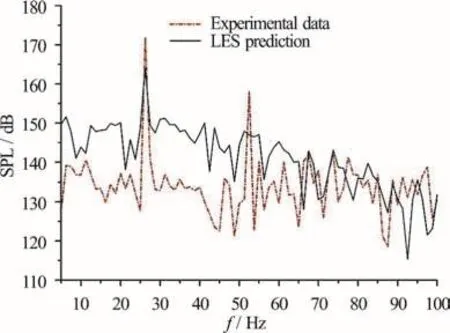
Fig.18 (Color online) The numerical and experimental results of the unsteady pressure spectra, =2.6 m/s

Two empirical constants are in this equation: α,depending on the dimension of the orifice, andck,depending on the Mach number. The values of the coefficients α andck are taken from Ref. [1] as 0.25 and 0.53, respectively. Furthermore, in view of the low Mach number, the fluctuating frequencies can be given by

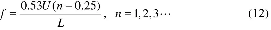
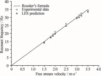
Fig.19 Comparison between measuredand predictedfirst Rossiter’s frequencies at different free stream velocities

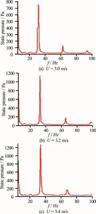
Fig.20 (Color online) Measured pressure fluctuations with the orifice open at different free stream velocities

For the cavity geometry used in this study, the frequency for the first Rossiter’s mode (n = 1) is. The sound pressure level (SPL) is calcu-lated based on a reference pressure pref=1μ Pa .Figure 18 shows the numerical and experimental results of the unsteady pressure spectra at a free stream velocity of U =2.6 m/s . The high intensity peaks at 26 Hz correspond to the frequency of the first Rossiter’s mode (n = 1) at 26 Hz. The frequency of the peak predicted by the LES is in good agreement with the experimental result, while the amplitude is smaller than the experimental result. The pressure fluctuations are induced by the interaction of the vortex in the cavity area, affected by the turbulence at the inflow boundary. However, the real inlet turbulence condition of the water tunnel is complex and difficult to measure. Without the information of the inlet turbulence condition, the amplitudes predicted by the numerical model, therefore, are smaller than the amplitudes obtained experimentally.

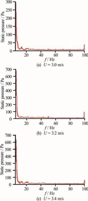
Fig.21 (Color online) Measured pressure fluctuations with the orifice closed at different free stream velocities

Figure 19 compares the measured and predicted first Rossiter’s frequency at different free stream velocities. In the experimental measurements, it is found that the pressure transducer cannot detect any significant pressure fluctuation when the free stream velocity is below 1m/s. One possible reason is that at a low free stream velocity, the amplitude of the pressure fluctuations is too small to be measured. Hence, the first Rossiter’s frequency at different free stream velocities, obtained numerically from the LES simulation and measured experimentally, are compared in the range from U =1.5-3.5 m/s . Figure 19 indicates that the numerical and experimental results are consistent with the Rossiter’s formula. Since the amplitude of the second Rossiter’s mode is small, so only the first mode is examined in the pressure fluctuations analysis. Figure 20 shows the measured pressure fluctuations with the orifice open at different free stream velocities. Figure 20 shows that with the increase of the free stream velocity, the resonant frequency increases linearly. When the orifice is closed, no peaks can be observed in the experimental results (Fig. 21).

These pressure fluctuations are very important for the vibro-acoustic analyses, as they represent the main sources exciting the vibration of the hydrofoil structure which radiates the underwater noise.

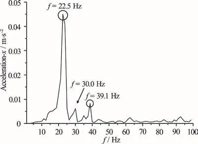
Fig.22 Numerical predictions of frequency response of x axis acceleration with the orifice open, U =3.1m/s

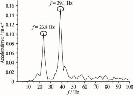
Fig.23 Numerical predictions of frequency response of x axis acceleration with the orifice closed, U =3.1m/s

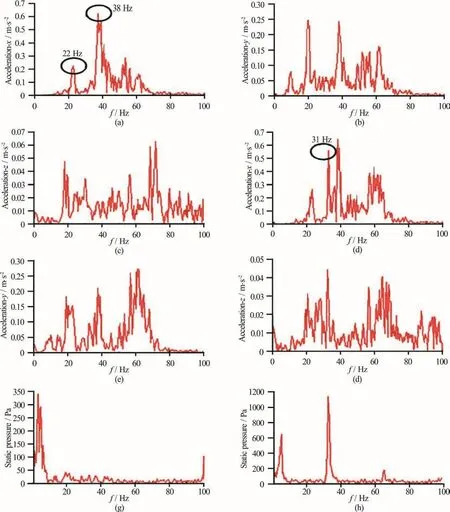
Fig. 24 (Color online) Measured acceleration responses and pressure spectra with orifice open and closed at U =3.1m/s

3.3 Vibration and sound radiation results

In what follows, the vibration and sound radiation results of the hydrofoil obtained numerically and experimentally are discussed and compared. In the vibration analysis, the acceleration response in the frequency domain of the hydrofoil is calculated at the node of the same location as the triaxial accelerometer on the hydrofoil side wall.

Figure 22 shows the numerical results of the frequency response with the orifice open at U =3.1m/s .The peaks at 22.5 Hz and 39.1 Hz correspond to the predicted first and third natural frequencies of the hydrofoil in water as shown in Table 2, res pectively.The peak at 30 Hz is excitedbythepressurefluctuations with a frequency equal to the first Rossiter’s frequency.

Figure 23 shows the numerical results of the frequency response with the orifice closed at =U 3.1m/s. The peaks at 23.8 Hz and 39.1 Hz correspond to the hydrofoil second and third natural frequencies in water as shown in Table 2, respectively. From Figs.22, 23, it can be seen that the pressure fluctuations induced by the flow over the cavity have a significant effect on the dynamic response of the hydrofoil structure. When the orifice is closed, the peak at 30 Hz disappears; the frequency response only shows the properties of the hydrofoil natural frequencies in water.

Figure 24 shows the experimental results measured by the triaxial accelerometer and the pressure transducer with the orifice open and closed, respectively. The peaks at 22 Hz and 38 Hz in Fig. 24(a)correspond to the hydrofoil second and third natural frequencies in water as shown in Table 2. From Figs.24(a), 24(d), it can be observed that the pressure fluctuations induced by the flow over the cavity excite the hydrofoil structure vibration. These excitations have a major frequency equal to the first Rossiter’s frequency, which can be predicted by the Rossiter’s formula or the LES.

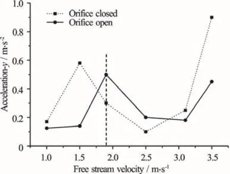
Fig.25 Measured y axis acceleration amplitudes at 19 Hz with orifice open and closed at various free stream velocities

Figure 25 shows the measured y axis acceleration amplitude at 19 Hz with the orifice open and closed at different free stream velocities. The resonance occurs at=1.9 m/s which corresponds to the first Rossiter’s frequency, 19 Hz. The pressure fluctuations excite the hydrofoil first mode in water,therefore an acceleration peak appears at U=1.9 m/s. In the case where the orifice is closed, one observes no resonance.

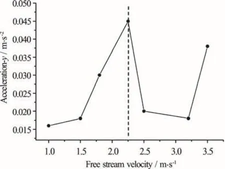
Fig.26 Numerical results of y axis acceleration amplitudes at 22.5 Hz with orifice open at various free stream velocities

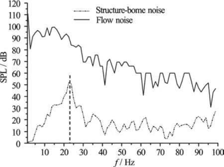
Fig.27 Numerical results of hydrofoil structure-borne noise and flow noise at U =3.1m/s

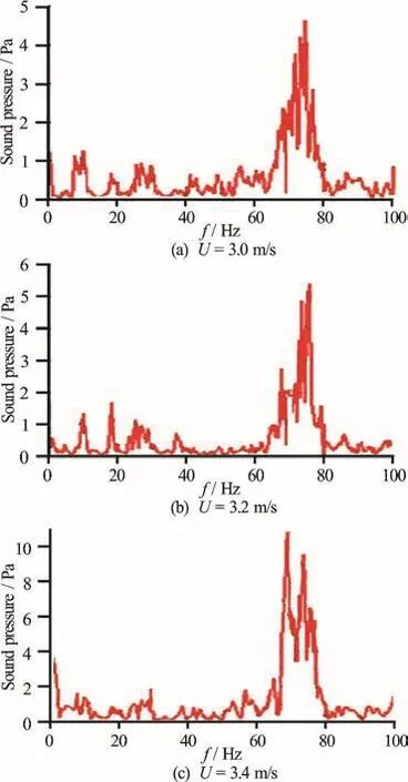
Fig.28 (Color online) The background noises in the water tunnel at different free stream velocities

The numerical results as shown in Fig. 26 also show this resonance phenomenon at 22.5Hz corresponding to the hydrofoil first mode in water. The experimental measurement and the numerical simulation both successfully reveal the resonance phenomenon caused by the interaction between the hydrofoil structure and the fluctuating flow. These results verify that the pressure fluctuations induced by the flow over a cavity have a significant effect on the vibration of the hydrofoil structure.

However, some discrepancies between the experimental and numerical simulation results are observed in the structural acceleration response. The amplitudes of the acceleration obtained by the numerical simulation are much smaller than those of the experimental measurement.

The main reasons why the numerical results are much smaller than the experimental results are as follows: (1) The numerical model has a high symmetry (the geometry, the flow field and the boundary conditions), while the experimental model does not.These kinds of asymmetry of the experimental model can increase the structural response when the hydrofoil is testing in a water tunnel. (2) The errors produced by the data transfer from the fluid mesh to the structural mesh. As the fluid mesh is not consistent with the structural mesh, the data should be transferred from the fine fluid mesh to the coarse structural mesh. The errors can be produced during this procedure. (3) The inlet turbulence condition. The pressure fluctuations of the cavity are induced by the interaction of the vortex, affected by the turbulence at the inflow boundary. However, the real inlet turbulence condition of the water tunnel is complex and difficult to measure. Without the information of the inlet turbulence condition, the amplitudes predicted by the numerical model, therefore, are smaller than the amplitudes obtained experimentally. This finally leads to the errors in the structural response calculations.

Furthermore, the sound radiation of the hydrofoil is discussed. This flow-induced noise consists of two parts, the structure-borne noise and the flow noise.The structure-borne noise is the direct sound radiation from the vibrational hydrofoil structure; while the flow noise is the sound radiation induced by the cavity surface pressure fluctuations. Figure 27 shows the numerical results of the hydrofoil structure-borne noise and the flow noise at U=3.1m/s. It can be found that the flow noise is higher than the structure-borne noise. The structure-borne noise has a significant peak at 22.5 Hz corresponding to the hydrofoil first mode in water, implying that the hydrofoil first mode in water contributes to the peak in the structure-borne noise spectra. From the results, it is difficult to find any correlation between the flow noise and the Rossiter’s frequencies.

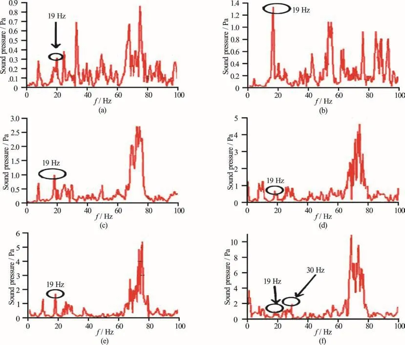
Fig. 29 (Color online) Measured sound pressures by the hydrophone at different free stream velocities

Figure 28 shows the background noise in the water tunnel at different free stream velocities. Figure 29 shows the measured sound pressure spectra with the hydrofoil in the water tunnel. From these two figures, it can be seen that, with the increase of the free stream velocity, the measured sound pressure increases. High intensity peaks around 72 Hz can be found in all cases. These peaks are found to be highly correlated to a longitudinal acoustic mode in the water tunnel which is easily excited by the flow turbulence inside the tunnel. Under the idealized conditions of the water tunnel at a constant flow velocity, the frequency of the longitudinal acoustic modes of the water tunnel is given by the relation[18]

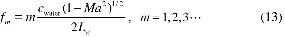
where cwateris the sound speed in water, Lwis the length of the water tunnel working segment10.6 m).

For the present water tunnel, the first mode frequency (m = 1) is 70.7 Hz, which is very close to the measured peak frequency around 72 Hz. The peaks at 19 Hz is identified as the structure-borne noise, for they have a frequency corresponding to the hydrofoil first mode in water and have a maximum amplitude at U=2m/s (Fig. 29(e)). When the free stream velocity is close to 1.9m/s, the resonance occurs and the hydrofoil structural acceleration reaches the maximum amplitude, meantime the hydrofoil radiates a highest structure-borne noise at 19 Hz as indicated in Fig. 27. However, when the free stream velocity is 3 m/s (Fig. 29(f)), the peak at 30 Hz is higher than the peak at 19 Hz. The peak at 30 Hz is identified as the flow noise, for it has the same frequency as the first Rossiter’s frequency. It can be found that at a low free stream velocity, the total radiated noise is dominated by the structure-borne noise, while at U = 3the flow noise is higher than the structure-borne noise. The flow noise simply increases with the increase of the free stream velocity,while the variation of the structure-borne noise depends on the structural vibration pattern of the cavity.

4. Conclusions

This paper presents an experimental and numerical study of the structural vibration and the sound radiation induced by the flow over a hydrofoil with a cavity. The numerical simulations are validated with experimentally measured modes in air and water, in addition to the measured pressure spectra, the structural vibrational response in the frequency domain and the sound radiation in a water tunnel. In general,reasonable agreements are observed between the numerical predictions and he experimental measurements. The following concluding remarks can be made:

(1) The natural frequencies of the first and second order modes of the hydrofoil are shown to be significantly affected by the heavy fluid loading.

(2) The prediction of the pressure fluctuations over the cavity of the hydrofoil can be made with a reasonable accuracy by a modified Rossiter’s formula or the LES. The first order Rossiter’s mode dominates the pressure fluctuations.

(3) The pressure fluctuations over the cavity are found to excite the hydrofoil vibration. Resonance is observed to occur when the cavity’s first order Rossiter’s frequency is equal to the frequency of the hydrofoil first order mode in water.

(4) At a low free stream velocity (less than 3 m/s),the total sound radiation is dominated by the structureborne noise of the hydrofoil, which highly depends on the structural vibration. The flow noise increases with the increase of the free stream velocity and is greater than the structure-borne noise at 3 m/s.