Directed Dominating Set Problem Studied by Cavity Method:Warning Propagation and Population Dynamics∗
2018-12-13YusupjanHabibulla玉素甫艾比布拉
Yusupjan Habibulla(玉素甫·艾比布拉)
School of Physics and Technology,Xinjiang University,Sheng-Li Road 14,Urumqi 830046,China
AbstractThe minimal dominating set for a digraph(directed graph)is a prototypical hard combinatorial optimization problem.In a previous paper,we studied this problem using the cavity method.Although we found a solution for a given graph that gives very good estimate of the minimal dominating size,we further developed the one step replica symmetry breaking theory to determine the ground state energy of the undirected minimal dominating set problem.The solution space for the undirected minimal dominating set problem exhibits both condensation transition and cluster transition on regular random graphs.We also developed the zero temperature survey propagation algorithm on undirected Erd˝os-Rényi graphs to find the ground state energy.In this paper we continue to develope the one step replica symmetry breaking theory to find the ground state energy for the directed minimal dominating set problem.We find the following.(i)The warning propagation equation can not converge when the connectivity is greater than the core percolation threshold value of 3.704.Positive edges have two types warning,but the negative edges have one.(ii)We determine the ground state energy and the transition point of the Erd˝os-Rényi random graph.(iii)The survey propagation decimation algorithm has good results comparable with the belief propagation decimation algorithm.
Key words:directed minimal dominating set,replica symmetry breaking,Erd˝os-Rényi graph,warning propagation,survey propagation decimation
1 Introduction
The minimum dominating set for a general digraph[1−2]is a fundamental nondeterministic polynomialhard(NPhard)combinatorial optimization problem.[3]Any digraph D=V,A contains a set V≡1,2,...,N of N vertices and a set A≡{(i,j):i,j∈V}of M arcs(directed edges),where each arc(i,j)points from a parent vertex(predecessor)i to a child vertex(successor)j.The arc density α is defined by α ≡ M/N.A directed dominating set Γ is a vertex set such that,for any node in the network,either the node itself or one of its predecessors belongs to Γ.A directed minimal dominating set(DMDS)is a smallest directed dominating set.The DMDS problem is very important for monitoring and controlling the directed interaction processes[4−10]in the complex networks.
The statistical physicists have widely studied this optimization problem using the statistical physics of spin glass systems.[11−19]The cavity method is used to estimate the occupation probability at each node,and a solution for the given problem is constructed using this probabilities.Using statistical physics does not always yield a single solution for a given graph,but if this graph does not contain any small loops,then the cavity equation may converge to a stable point,so we can study the problem using the cavity method.
Research into spin glass systems can be divided into two levels-the replica symmetry(RS)level and the replica symmetry breaking(RSB)level.For a given optimization problem,RS theory finds the smallest set in the given graph that satisfy this problem,and RSB theory finds the number of solutions and the ground state energy.Previously,we have found the smallest minimal dominating set(MDS)using the cavity method on both directed and undirected networks,[20−21]and have found the ground state energy for undirected networks.[22]The current study is inspired by Ref.[22],where we studied the ground state energy for the DMDS problem also using the cavity method.At a temperature of zero,we used survey propagation to find the ground state energy of the Erd˝os-Rényi graph(ER)random graph.
This paper studies the solution space of the DMDS problem using one step replica symmetry breaking(1RSB)theory from statistical physics.This work is a continuation of our earlier work[22]on the solution space of the undirected MDS problem.We organize the paper as follows.In Sec.2,we recall RS theory for spin glass systems before introducing RSB theory.We present the belief propagation(BP)equation,thermodynamic quantities and warning propagation for the DMDS problem.In Sec.3,we introduce 1RSB theory and the associated thermodynamic quantities.We then derive 1RSB theory and thermodynamic quantities at β = ∞,and survey propagation(SP)for the DMDS problem,before introducing the survey propagation decimation(SPD)process for the DMDS problem in detail.Finally in Sec.4 we conclusion our results.
2 Replica Symmetry
2.1 General Replica Symmetry Theory
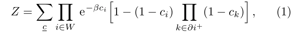
To estimate the MDS for a given graph using the way of mean field theory,we must have the partition function for the given problem.The partition function Z is
We use RS mean field theory,such as the Bethe-Peierls approximation[23]or partition function expansion,[24−25]to solve the above spin glass model.We assign the cavity messageon the every edge,and these messages must satisfy the equation
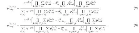
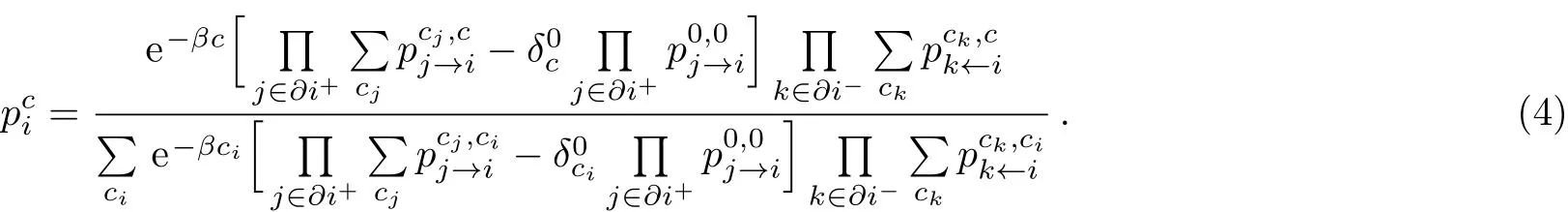
known as the BP equation.The Kronecker symbol is defined by=1 if m=n and=0 otherwise.The cavity messagerepresents the joint probability that node i is in state ciand the adjacent node j is in state cjwhen the constraint for node j is not considered.The marginal probabilityfor node i is expressed as
Finally the free energy can be calculated using mean field theory as

where

We use Fito denote the free energy at node i,and F(i,j)to denote the free energy of the edge(i,j).We iterate the BP equation until it converges to a stable point,and then calculate the mean free energy f≡F/N and the energy densityusing Eqs.(3)and(4).The entropy density is calculated as s= β(ω −f).
2.2 Warning Propagation
In this section,we introduce BP at β = ∞,which is called warning propagation.Even though the warning propagation may converge very quickly,it can only converge for C<3.704 on an ER random network,so we must further consider the 1RSB case at β = ∞.To estimate the minimal energy of an MDS,we must consider the limit at β = ∞.There are three cases for a single node:(i)node i appears in every MDS,namely=1,=0;(ii)node i appears in no MDS,namely=0,=1;(iii)node i appears in some but not all MDSs,namely=0.5,=0.5.Thus there are nine cases for the pair of nodes(i,j).However,only four cavity messages are possible:(i)node i appears in every MDS and node j appears in some but not all MDSs,namelynode i appears in no MDS and node j appears in some but not all MDSs,namely(iii)node i appears in no MDS and node j appears in every MDS,namely(iv)node i appears in some but not all MDSs and node j appears in some but not all MDSs,namely
The other five cases do not satisfy the normalization condition:(i)if node i appears in every MDS and node j appears in every MDS,namely,then from the relationshipwe can deriveso that the total probability is greater than 1,which is not possible;(ii)if node i appears in every MDS and node j appears in no MDS,namely,then in the same way we can derive,so the total probability is again greater than 1;(iii)if node i appears in some but not all MDSs and node j appears in every MDS,namely,then(iv)if node i appears in some but not all MDSs and node j appears in no MDS,namelythenif node i appears in no MDS and node j appears in no MDS,namely,then from Eqs.(2)and(3)we see thatis always smaller thanand does not exceed 0.5.It is good to understand that if a node is not occupied,then it cannot request any of its neighbors to be unoccupied in the MDS problem.On the other hand,if a node is occupied,then it cannot request any of its neighbors to be either occupied or unoccupied.There is one warning message pi→j=0 for a single node,but there are two warning messages for a pair nodes(i,j),that is,andThe warning messageis called a first type warning,and the warning messageis called a second type warning.
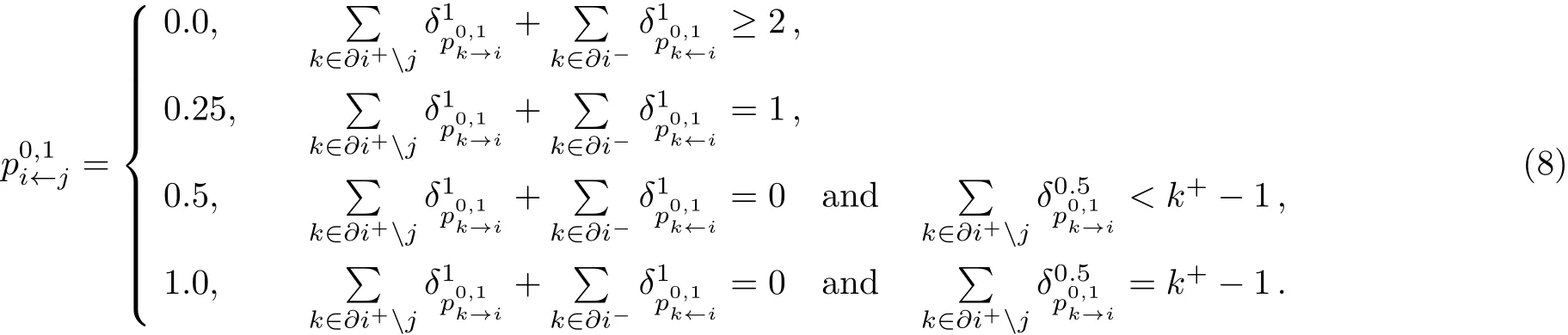
If node i is not covered or observed,so the neighbor node j must be covered,the corresponding case isIf node i is not covered,but it has been observed,so node j can be covered or uncovered,namely.So we can easily understand the upper equation.In the first line,if two or more neighbors(successors exactly)of the node i are not covered or observed,then we must cover the node i to observe them,namelyorIn the second line,if only one neighbor(successor exactly)of the node i is not covered or observed,then we have both opportunity to cover or uncover the node i,namelyor.In the third line,if every successor of the node i is observed,but it is observed predecessors less than k+−1,then we must not cover the node i,the neighbor j can be covered or uncovered,namelyor.In the fourth line,if every successor of the node i is observed,but the every predecessors of the node i are observed except node j,so we must not cover the node i,and the neighbor j must be covered,namelyWe can find that only the successor nodes provide the first type warning,in the same way we can read the following equation
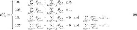
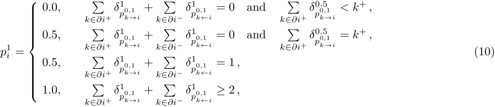
The above equations are called warning propagation equations.Only the messagecan produce a first type warning when the incoming messages do not include any first type messages and the incoming positive messages have∂i+− 1 second type messages.If we find the stable point of the warning propagation,then we can calculate the coarse-grained state of every node as
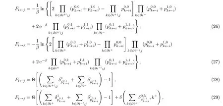
and we can calculate the free energy for the DMDS problem in the general case as

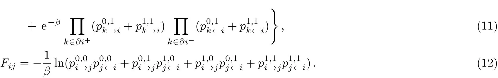
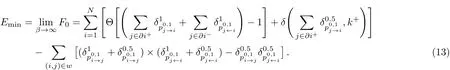
The energy equals the free energy when β = ∞,so from the above questions we can write the free energy and the energy as
The warning propagation convergence speed is very fast,and gives the same results as BP,but it does not converge when the mean variable degree is greater than 3.704 on the ER random graph.For some single graphs,the convergence degree is greater than 3.704,but it is very close to 3.704 in most single graph networks.
3 One Step Replica Symmetry Breaking Theory
In this section,we introduce 1RSB theory for spin glass systems,which is calculated using the graph expansion method.We first introduce the generalized partition function,free energy,SP,grand free energy and complexity in the general case.To obtain the ground state energy,we must consider the limiting behavior of the DMDS problem at β = ∞,so we next derive the simplified equations at β=∞for the DMDS problem,and then introduce the numerical simulation process for population dynamics.
3.1 General One Step Replica Symmetry Breaking Theory
The RS theory only finds low energy configurations.To study the subspace structure for a given problem,researchers have been developing 1RSB theory.In 1RSB theory,our order parameter is a free energy function.At higher temperatures,the microscopic thermodynamic state consisting of some higher energy configurations determines the statistical physics properties of the given system,and the subspace of this microscopic state is ergodic.However,at lower temperatures the microscopic state is no longer ergodic but is divided into several subspaces,and the contribution of these subspaces to the equilibrium properties are not the same.We define the generalized partition function Ξ by
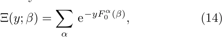
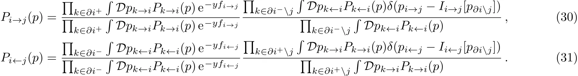
We use α to denote the microscope states that achieve the minimum free energy,and thushas the following form:
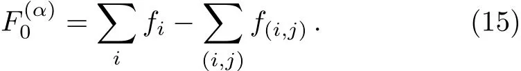

The notation Ii→j[p∂ij]is short-hand for messages updating equation(2),and Ii←j[p∂ij]is short-hand for messages updating equation(3).The weight free energies fi→jand fi←jare respectively equal to

The generalized free energy density g0is
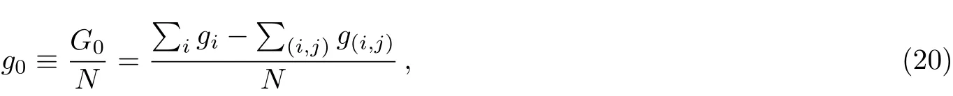
where


We further have the mean free energy density

where
Finally,with mean free energy〉and generalized free energy g,we derive the complexity as
3.2 Coarse-Grain Survey Propagation
We next derive the SP for the case β = ∞and estimate the ground state energy,and then predict the energy density using the SPD method.We find that the SP results fit with the SPD results,which are as good as the belief propagation decimation(BPD)results.To obtain the SP,we must know the form of the free energy Fi→jat a temperature of zero.From the general form,we can derive the free energy Fi→jas
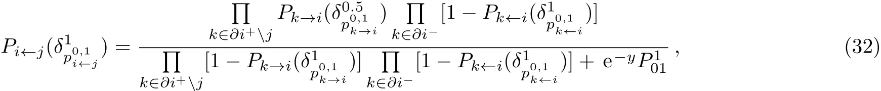
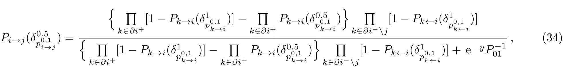
the survey propagation for general case as
We can obtain the SP at a temperature of zero using Eqs.(28)–(31)as


and the grand free energy of node i and edge(i,j)for the general case as

From Eqs.(35)–(38),we can derive the grand free energy of node i and edge(i,j)at a temperature of zero as

where

the grand free energy density is

The free energy of the macroscopic state α when β = ∞ has several different ground state energies Emin,we cannot calculate the ground state energies one at a time.We are only concerned with the average ground state energy,so we focus our discussion on this.We denote the microscopic average minimal energy by 〈Eβ=∞〉,which is calculated using the following equation:
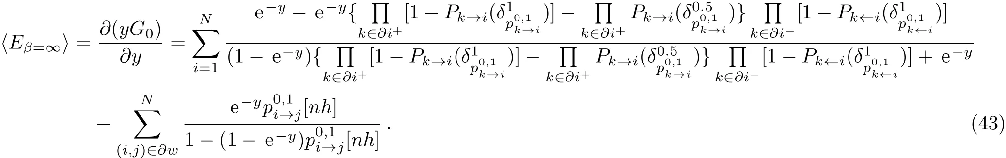
We can study the ensemble average properties of the DMDS problem using population dynamics and Eqs.(28)–(31),(37)and(38).Figure 1 indicates the results of the ensemble everage 1RSB population dynamics for the DMDS problem on the ER random graph with mean connectivity C=5.The complexity∑=0 at y=0,and the complexity is not a monotonic function of the Parisi parameter y.It increases as the Parisi parameter y increases,and reaches its maximum value when y≈3.7.The complexity then begins to decrease as y increases and becomes negative when y≈8.35.From Fig.1,we can see that there are two parts to the complexity graph when it is a function of energy,but because of only the concave part is decline function of energy,so it has the physical meaning.The grand free energy is not a monotonic function of y either.It reaches a maximum when the complexity becomes negative at y≈8.35,so the corresponding energy density u=0.3212 is the minimum energy density for the DMDS problem at this mean connectivity.

Fig.1 The 1RSB results for the zero temperature DMDS problem on the ER random graph with mean connectivity c=5 using population dynamics.In the upper two and bottom left graphs,the x-axis denotes the Parisi parameter Y,and the y-axis denotes the thermodynamic quantities.The complexity becomes negative when the Parisi parameter is approximately 8.35.At this point,we select the corresponding energy as the ground state energy,which equals 0.3212.In the bottom right graph,the x-axis denotes the energy density and the y-axis denotes the complexity.
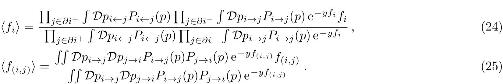
We can calculate some microscopic statistical quantities using Eqs.(32)–(34)at a temperature of zero.For example,for the probability(statistical total weight of all macrostates)of the variable staying in a coarse grained state,we use pi(0)to denote the probability of the variable staying in a totally uncovered state,pi(1)to denote the probability of the variable staying in a totally covered state,and pi(∗)to denote the probability of the variable staying in an unfrozen(some microstates covered)state.We can derive the representation of these three probabilities using 1RSB mean field theory as

Using the 1RSB population dynamics,we obtain the minimal energy densities for ER random network ensembles with different mean connectivities.In Table 1,we list the theoretical computational results for C≤10.We can see that the ground state energy and transition point depend on the mean connectivity C.From Ref.[22],we know that the transition point does not depend on the mean connectivity C in undirected networks.
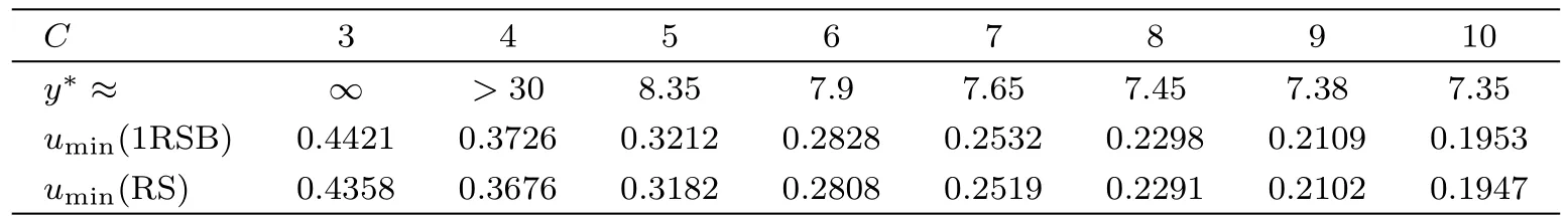
Table 1 The parisi parameter y∗transition point and the ground state energy for ER random graphs.
In these simulations,we update the population MI=1000 times.That is,we update each element in the population 1000 times on average to reach a stable point for the population,and sample MS=5000 times to obtain the transition point of∑(second∑=0 points)and the corresponding ground state energy value Eminon the ER random graph.The cluster transition point is only correct when the Parisi parameter sample distance is▽y≥ 0.1,but the ground state energy is correct in any small enough Parisi parameter sampling distance with a precision of▽E=0.0001.We use two types of population,a positive population and a negative population,and set the population size to N=1 000 000.Increasing the number of updates or the number of samples does not affect the simulation results.However,increasing the population size N used to calculate the thermodynamic quantities improves the results.Within a sampling distance of▽y=0.1,we can also obtain good results with fewer updates.However,with a sampling distance of▽y=0.01,we need an increasing number of updates to obtain good results.The required numbers of updates and samples increases as the variable degree decreases.
3.3 Survey Propagation Decimation
We studied undirected networks using SP in Ref.[22].We can also study the statistical properties of microscopic configurations in a single directed network using the SP in Eqs.(32)–(34).The results are similar to those for an undirected network.For example,SP can find a stable point for a given directed network easily when the Parisi parameter y is small enough,and we can then calculate the thermodynamic quantities using Eqs.(35),(36),and(39)–(42).However,SP does not converge when y is too large.For example,SP does not converge when y≥7 for an ER random network when C=10.We have already discussed the reasons for this in undirected network in Ref.[22],namely that the coarse-grained assumption and 1RSB mean field theory are not sufficient to describe microscopic configuration spaces when the energy is close to the ground state energy,so a more detailed coarse-grained assumption and a higher-level expansion of the partition function are required.For further discussion of convergence of coarse-grained SP,see Refs.[26–27].
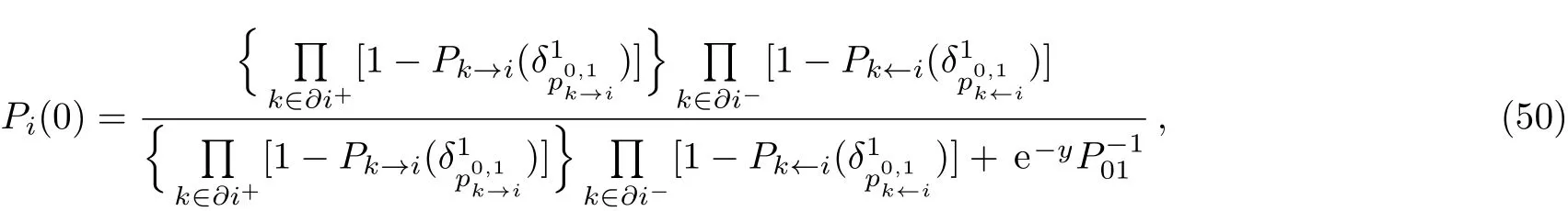
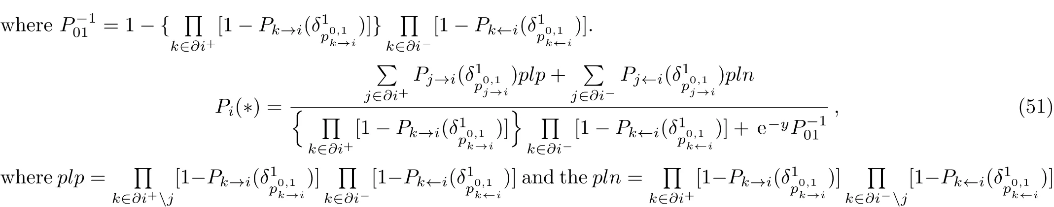
We can construct one or more solutions that are close to the optimal DMDS for a given graph W using 1RSB mean field theory.One very efficient algorithm is the SPD algorithm.[22,26−27]The main idea of this algorithm is to first determine the probability of being covered,and then select a small subset of variables that has the highest probability of being covered.We then set the covering probability for this subset of variables to ci=1,and delete all variables for which the covering probability equals 1,along with the adjacent edges,and then simplify the network iteratively.If a node i is unobserved(it is empty and has no adjacent occupied parent node),then the output messages Pi→jand Pi←jare updated according to Eqs.(32)–(34),On the other hand,if node i is empty but observed(it has at least one adjacent occupied parent node),then this node presents no restriction on the occupation states of its unoccupied parent neighbors.For such a node i,the output messages Pi→jand Pi←jare then updated according to the following equations:
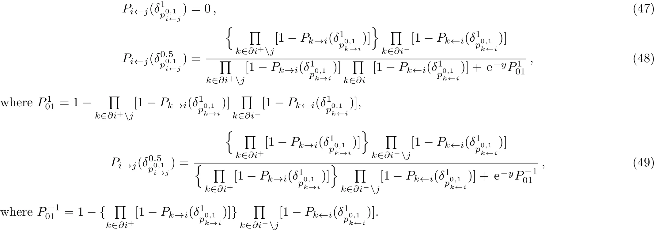
As with Eqs.(47)–(49),the marginal probability distribution Pifor an observed empty node i can be evaluated according to

We now present the details of this algorithm.
(i)Read the network W,set the covering probability of every vertex to uncertain,and define four coarsegrained messages,andon each edge of the given graph.Randomly initialize the messages in the interval(0,1],ensuring that for every pair of messagesand,the normalization conditionsandare satisfied.An appropriate setting for the macroscopic inverse temperature y is a value close to the threshold value.For example,if SP does not converge when y≥3.01,then we set y=3.
(ii)Iterate the coarse-grained SP equations(Eqs.(32)–(34)or Eqs.(47)–(49)),for L0steps,aiming for convergence to a stable point.At each iteration,select one node i and update all messages corresponding to node i.After updating the messages L0times,calculate the coarsegrained probability(Pi(1),Pi(∗),Pi(0))using Eqs.(44)–(46)or Eqs.(50)–(52).
(iii)Sort the variables that are not frozen in descending order according to the value of Pi(1).Select the first r percent to set the covering state as ci=1,and add these variables to the DMDS.
(iv)Simplify the network by deleting all the edges between the observed nodes and deleting all the occupied variables.If the remaining network still contains one or more leaf nodes,[20]then apply the GLR process[21]until there are no leaf nodes in the network and simplify the network again.This procedure is repeated(simplify-GLR-simplify)until the network contains no leaf nodes.If the network contains no nodes and no edges,then stop the program and output the DMDS.
(v)If the network still contains some nodes,then iterate Eqs.(32)–(34)or Eqs.(47)–(49)for L1steps.Repeat steps(iii),(iv),and(v).
Figure 2 shows the numerical results of the SPD algorithm on an ER random graph.We can see that the SPD results are very close to the BPD results,and thus the SPD algorithm finds an almost optimal solution.We perform the BPD algorithm as detailed in Ref.[20].
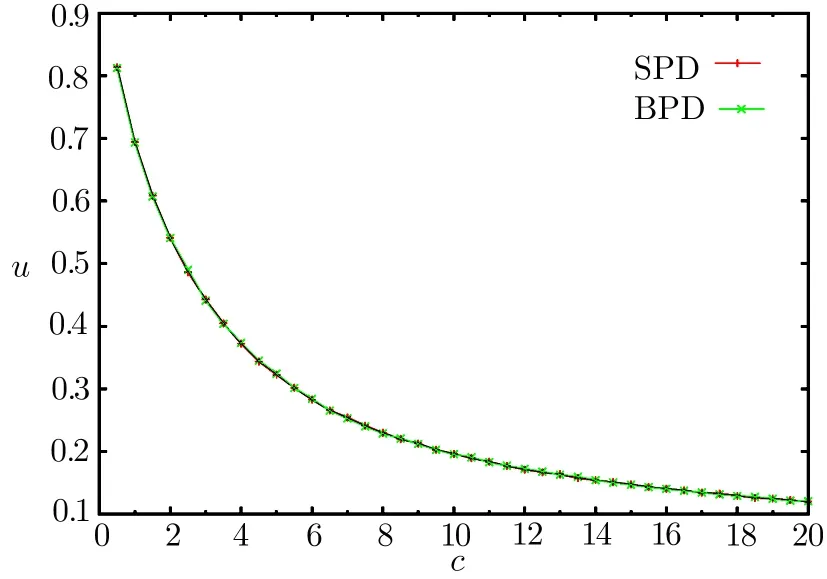
Fig.2 The solid line is the result of the SPD algorithm,and the crosses are the results of the BPD algorithm.Our simulation was performed on an ER random graph with 104variables.
4 Discussion
In this work,we first derived the warning propagation and proved that the warning propagation equation only converges when the network does not contain a core.[21]There is only one warning in the vertex cover problem,[28]but the MDS problem has two warnings.In the DMDS problem,a positive edge pi←jhas two warnings,but a negative edge pi→jhas one warning.The reason for this is that each nodes only requires the parent nodes,not child nodes,to be occupied to be able to observe itself,so only the psitive edges have first type warnings.Second,we derived the SP equation at a temperature of zero to find the ground state energy and the corresponding transition point of the macroscopic inverse temperature.The change rules of the transition point do not like with undirected MDS problem.It is a monotonic function of the mean variable degree in the DMDS problem,but not in the undirected MDS problem.[22]The corresponding energy of the transition point Parisi parameter Y equals the threshold value xc,namely EY=xc.We then implemented the SPD algorithm at a temperature of zero to estimate the size of a DMDS.The results are as good as the BPD results.
We have previously studied the MDS problem on undirected networks and directed networks using statistical physics,and more recently we studied the undirected MDS problem using 1RSB mean field theory.We have now studied the DMDS problem using 1RSB theory.We plan to study the MDS and DMDS problems using long range frustration theory in the future.
Acknowledgement
Yusupjan Habibulla thanks Prof.Haijun Zhou for helpful discussions and guidance.Yusupjan Habibulla also thanks Prof.Xiaosong Chen for helpful discussions and support.We implemented the numerical simulations on the cluster in the School of Physics and Technology at Xinjiang University.We thank Peter Humphries,PhD,from Edanz Group(www.edanzediting.com/ac)for editing a draft of this manuscript.
杂志排行

Communications in Theoretical Physics的其它文章
- Electron Transport Properties of Graphene-Based Quantum Wires∗
- Magnetic Properties of XXZ Heisenberg Antiferromagnetic and Ferrimagnetic Nanotubes∗
- On the Singular Effects in the Relativistic Landau Levels in Graphene with a Disclination∗
- Super-sensitivity in Dynamics of Ising Model with Transverse Field:From Perspective of Franck-Condon Principle∗
- New Feedback Control Model in the Lattice Hydrodynamic Model Considering the Historic Optimal Velocity Di ff erence Effect∗
- A Class of Rumor Spreading Models with Population Dynamics∗