Review：A Critical Assessment on the Predictability of 14Micromechanics Models for the Stiffness and Strength ofUD Composites

Zhengming Huang and Chunchun Zhang

(School of Aerospace Engineering &Applied Mechanics, Tongji University, Shanghai 200092, China)

Abstract: Any micromechanics model initially developed for predicting stiffness (elastic property) of a composite can be used to predict its strength with a reasonable accuracy, as long as the homogenized stresses in the matrix are converted into its true values. A critical assessment on the predictability of 14 famous micromechanics models for stiffness and strength of UD (unidirectional) composites was made in this work against the benchmark data provided in three world-wide failure exercises (WWFEs). Bridging Model exhibited the highest accuracy in both the stiffness and strength predictions. Moreover, it was the only consistent model in the internal stress calculation. Non-consistency implies that a full three-dimensional (3D) approach should be used to predict the effective property of the composite. The paper also showed that the smallest fiber volume in an RVE (representative volume element) led to the best approximation to a composite property.

Keywords: composite; mechanical properties; micromechanics; stress concentration factors; true stress; RVE; consistency

1 Introduction

Fiber reinforced composites have been used in many engineering areas especially in aerospace industry. A main drawback in the use of composite materials is that their mechanical properties due to the influence of anisotropy have to be determined by difficult or expensive experiments. Micromechanics is a theory to approach the effective properties of a composite from its constituent information, which significantly reduces the demands on the experiments.

Numerious existing miromechanics models[1-3]are mainly developed for the prediction of a composite stiffness. Failure and strength behavior of the composite is hardly predictable only based on the original constituent data with a reasonable accuracy, according to Ref.[4]. By “original”, it means that the properties are either measured from monolithic material, for instance, matrix, specimens or ones documented in a recognized material database. Very recently, we have found that the homogenized stresses in the matrix of a composite determined by a micromechanics theory must be converted into true values before a failure assessment can be made against the original constituent properties[5-11]. The conversion is achieved by multiplying the homogenized quantities with corresponding stress concentration factors (SCFs) of a matrix in the composite. Such an SCF cannot be defined following a classical approach. Explicit formulae for the SCFs under various loads have been obtained[5-11], making a reasonable prediction for a composite strength achievable only by using the original constituent properties.

A critical assessment for the predictability of 14 well-known micromechanics models for the stiffness and more importantly for the strength of a UD composite is made in this paper. Previous comparisons, such as by Refs. [12-14], were made only for predicting stiffness by different models. Few has been found for the strength prediction. The models included in this paper are Eshelby’s method[15], Bridging Model16], Mori-Tanaka method[17-18], rule of mixture method[19], Chamis model[20], modified rule of mixture method[19], Halpin-Tsai formulae[21], Hill-Hashin-Christensen-Lo model[22], self-consistent method[15], generalized self-consistent method[15,23], double inclusion method[3], generalized method of cells (GMC)[24], generalized finite volume method (GFVM)[25-26], and finite element method (FEM)[27]. The measured stiffness and strength data of all the 9 independent UD composites in three WWFEs were used as benchmark to judge the prediction accuracy of each model. An accuracy ranking was made based on the overall correlation error between the predictions and the experiments. On the whole, Bridging Model exhibited the highest prediction accuracy in both stiffness and strength for the composites.

As solution of a numerical micromechanics method, GMC, GFVM, and FEM, depend on an RVE geometry to be discretized,different fiber arrangement patterns in the RVE have been chosen for the FEM solution. Many people deemed that a sufficient number of fibers arranged in a random pattern should be taken for an RVE[28-30], but this is not supported by our study. Among the four patterns, i.e. the square, hexagonal, square-diagonal, and the random fiber arrays, the smallest fiber volume or the square fiber array in the RVE resulted in the highest simulation accuracy. The conclusion is, in fact, easy to understand. By definition, the volume of an RVE, on which a homogenization is made, should be infinitesimal. Though in reality an RVE has to be finite, the smallest volume should lead to the best approximation, providing that all of the other conditions remain unchanged.

Finally, consistency is an issue that should be taken into account especially when a numerical micromechanics model is applied to simulate a composite property. Any model results in two sets of formulae, i.e. 2D and 3D formulae, for the internal stresses in the fiber and matrix. When the composite is subjected to a plane load, either the 2D or the 3D formulae can be applied to calculate the internal stresses. If the stress components by the 2D and the 3D formulae are exactly the same, the model is said to be consistent in the internal stress calculation. Among the 14 theories considered, only Bridging Model is consistent in this respect, implying that the full 3D approach of any other model investigated in this paper should be used to achieve the highest accuracy.

2 Internal Stress Determination

A composite is heterogeneous by nature. Any stress (as well as strain) should be defined based on averaged quantities with respect to its RVE of a volumeV′ through

(1)

It must be noted that by definitionV' is infinitesimal. A resulting stress, with "" on top, represents a point-wise quantity. IfV′ is finite, the corresponding stress is called a homogenized one. In Eq. (1),Vis a volume fraction withVf+Vm=1. A super-/sub-scriptformrefers to the fiber or matrix, whereas a quantity without any suffix stands for the composite.

(2)

(3)

Vm[Aij])-1

(4)

(5)

Thus, the prediction of the elastic moduli is equivalent to the calculation of the internal stresses in the fiber and matrix of the same composite.

3 Summary on Micromechanics Models

For the purpose of completeness, all the micromechanics models considered in this paper, except for the double inclusion method which has been incorporated into Digimat[31], are briefly summarized as follows.

3.1 Eshelby’s Method

The stiffness tensor of the composite by this method is given by[15]

(6)

(7.1)

(7.2.1)

(7.2.2)

L1212=L1313=1/4

(7.2.3)

(7.2.4)

(7.2.5)

whereνmis Poisson’s ratio of the matrix.

3.2 Bridging Model

The homogenized internal stresses by Bridging Model are expressed as[16]

(8.1)

(8.2)

ij=22, 33, and 23

(8.3), (8.4)

ij=12 and 13

(8.5), (8.6)

(9.1)

(9.2)

(9.3)

(9.4)

3.3 Mori-Tanaka Method

Non-zero bridging tensor elements of Mori-Tanaka method are given below[32]:

(10.1)

(10.2)

(10.3)

(10.4)

(10.5)

(10.6)

(10.7)

3.4 Rule of Mixture Model

Five elastic moduli of the composite defined by the rule of mixture model are[19]

(11.1)

(11.2)

(11.3)

(11.4)

(11.5)

3.5 Chamis Model[20]

(12.1)

(12.2)

(12.3)

(12.4)

(12.5)

3.6 Modified Rule of Mixture Model[19]

(13.1)

(13.2)

(13.3)

(13.4)

(13.5)

(13.6)

(13.7)

3.7 Halpin-Tsai’s Formulae[21]

(14.1)

(14.2)

(14.3)

(14.4)

(14.5)

(14.6)

3.8 Hill-Hashin-Christensen-Lo Model [22]

(15.1)

(15.2)

(15.3)

(15.4)

(15.5)

(15.6)

(15.7)

(15.8)

(15.9)

(15.10)

It is noted that Eq. (15.6) is applicable only to composites with isotropic fiber reinforcement.

3.9 Self-Consistent Method

The self-consistent formulae are represented as follows[15]:

(16.1)

(16.2)

(16.3)

(17.1)

(17.2)

(17.3)

(17.4)

(17.5)

(17.6)

(17.7)

Different from the preceding 8 explicit models, the self-consistent model is implicit. An iteration has to be carried out to determine the five effective elastic moduli of the composite,E11,E22,G12,ν12, andν23.

3.10 Generalized Self-Consistent Method

Fig. 1(a) Schematic for generalized self-consistent method, (b) Three-phase CCA model (b) for the generalized self-consistent method

(18)

The remaining three methods, GMC, GFVM, and FEM, belong to the approach of computational micromechanics, in which discretization on an RVE is necessary. Various selections of the RVE geometry have been used by different researchers. In this paper,the discretization scheme described in Ref.[35] is used. An RVE with a square fiber arrangement is applied to model a UD composite.

4 Assessment on Stiffness Prediction

Hinton et al.[4]organized three WWFEs to judge efficiency of the current strength theories for composites. A total number of 9 independent material systems were used. Mechanical properties of the fibers and matrices as well as fiber volume fractions of the 9 UD composites were provided[36-38], and are cited in Table 1. Measured effective properties of the composites from the exercise orginazors[36-38], which are used as a banchmark to assess the predicability of the 14 models, are listed in Table 2. Predictions for the five effective elastic moduli of each of the 9 UD composites by the 14 models were made and summarized in Table 3. Relative error of each prediction result in comparison with the measured counterpart (Table 2) was calculated, and the overall averaged errors by the 14 models are given in Table 4. Based on the overall errors, a ranking for the stiffness prediction accuracy is made and indicated in Table 4. It can be seen that Bridging Model exhibits overall the highest accuracy in the stiffness prediction. The second most accurate result was obtained by GFVM, which has a accuracy difference of 24% compared with Bridging Model. The similar conclusion can also be found in Refs. [12-14].

Table 1 Mechanical properties of the fibers and matrices of the 9 UD composites used in WWFEs[36-38]

It is acknowledged in the composite community that the prediction of the elasticity of UD composites is already mature. Thus, a significant improvement in the accuracy of both experimental measurement and micromechanics prediction for the elastic properties of a UD composite is not likely achievable. Considering the deviations occurred in the experimental measurement of the fiber, matrix, and composite properties and in light of Table 4, an attainable overall correlation error between the predicted and measured effective elastic moduli of the composite should be around 10%.

Table 2 Mechanical properties of the 9 UD composites used in WWFEs[36-38]

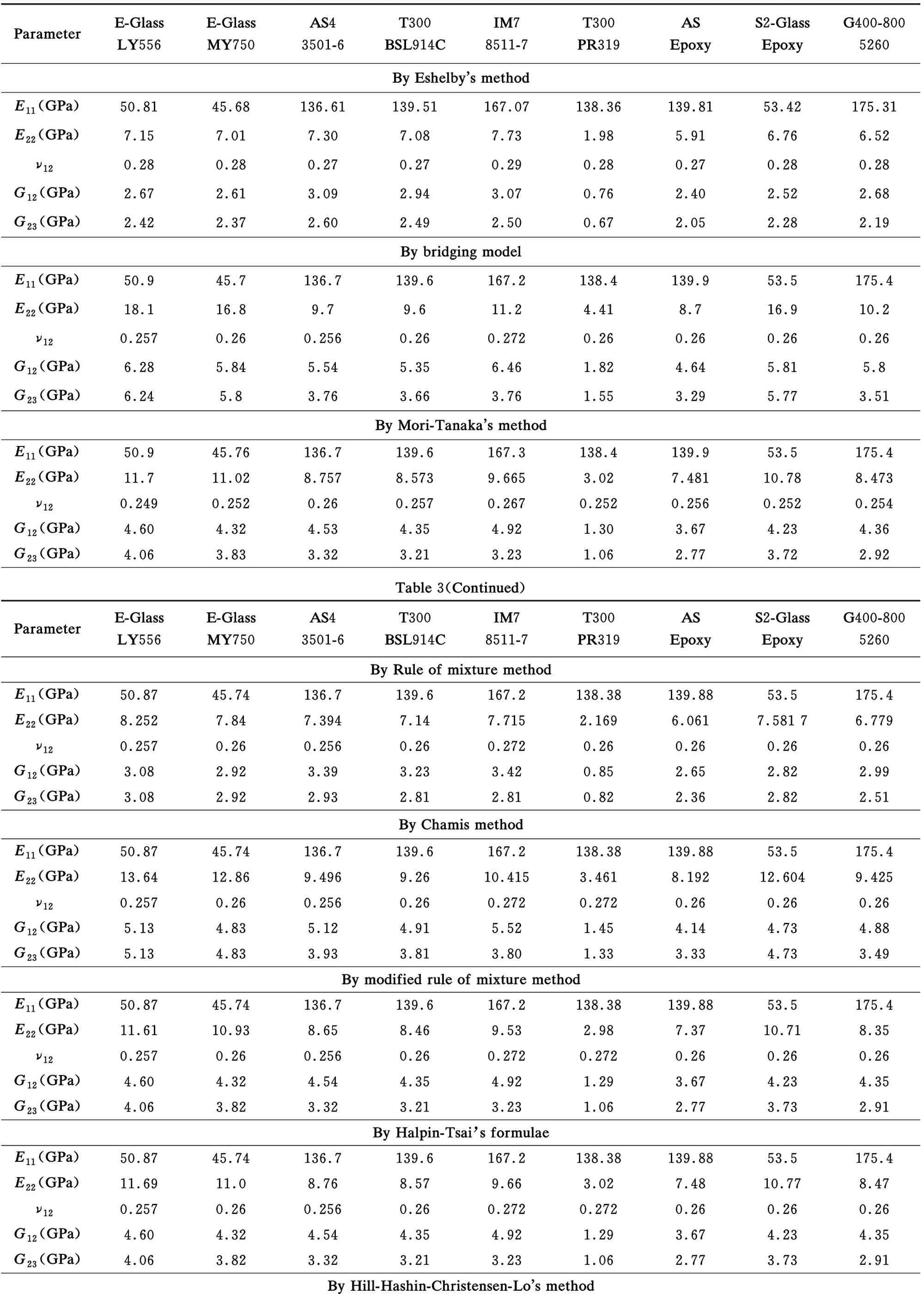
Table 3 Predicted elastic moduli of the 9 UD composites by different models

E11(GPa)50.945.8136.7139.6167.3138.4139.953.5175.4E22(GPa)12.912.0-----11.85-ν120.2490.2520.2530.2570.2670.2520.2560.250.25G12(GPa)4.64.324.544.354.921.293.674.234.35G23(GPa)4.654.33-----4.25-By self-consistent methodE11(GPa)50.9445.81136.72139.65167.31138.40139.9253.55175.43E22(GPa)18.9116.809.148.9910.374.198.0617.399.33ν120.2310.2350.2500.2540.2620.2380.2510.2330.247G12(GPa)11.349.806.376.259.364.185.8210.948.98G23(GPa)6.966.153.533.433.521.553.066.363.25By generalized self-consistent methodE11(GPa)50.945.8136.7139.6167.3138.4139.953.5175.4E22(GPa)12.8712.038.938.7710.13.277.7211.88.85ν120.2490.2520.2530.2570.270.250.2560.250.254G12(GPa)4.64.324.544.34.91.23.64.24.35G23(GPa)4.654.333.423.323.421.192.94.253.09By double-inclusion method (Digimat)E11(GPa)50.947.2141.1144.2172.8143144.555.2181.2E22(GPa)16.215.99.359.210.54.118.2616.19.48ν120.2340.2340.2480.2520.2570.2380.2490.2340.244G12(GPa)6.736.5855.85.637.122.1356.656.46G23(GPa)5.785.673.643.543.551.513.165.73.28Table 3(Continued)ParameterE-GlassLY556E-GlassMY750AS43501-6T300BSL914CIM78511-7T300PR319AS EpoxyS2-GlassEpoxyG400-8005260By FEM (FE-square fiber array)E11(GPa)50.945.8136.7139.6167.3138.4139.953.5175.4E22(GPa)16.2614.99.549.4210.883.988.4514.869.63ν120.2460.250.2520.2560.2660.250.2550.2490.252G12(GPa)4.964.584.684.55.151.383.824.54.57G23(GPa)6.495.893.793.713.791.583.325.893.47By GMC**E11(GPa)50.945.76136.7139.6167.3138.4139.953.5175.4E22(GPa)15.414.169.339.210.573.788.2114.099.35ν120.2470.2510.2530.2570.2670.2520.2560.2510.254G12(GPa)4.574.214.394.214.781.273.564.134.24G23(GPa)6.025.493.673.583.651.473.195.473.35By GFVM**E11(GPa)50.8945.76136.68139.6167.25138.36139.8853.5175.38E22(GPa)16.2614.99.539.4210.873.978.4414.869.62ν120.2460.250.2520.2560.2660.2510.2550.250.253G12(GPa)4.954.574.74.515.181.383.834.54.6G23(GPa)6.495.893.793.713.781.573.325.893.47By FE-hexagonal fiber array

E11(GPa)50.8945.77136.70139.56167.26138.38139.9053.50175.37E22(GPa)12.6011.728.898.729.893.197.6611.518.68ν120.2490.2510.2530.2550.2670.2590.2560.2510.252G12(GPa)4.624.324.544.354.911.303.674.224.35 G23(GPa)3.034.183.403.293.321.142.864.073.01By FE-square diagonal fiber arrayE11(GPa)50.8945.77136.71139.56167.30138.42139.8853.51175.43E22(GPa)10.409.858.308.099.032.717.129.607.92ν120.2480.2500.2510.2550.2640.2510.2600.2500.255G12(GPa)4.874.564.684.505.161.383.824.484.58G23(GPa)2.593.253.062.942.950.902.503.152.65By FE-random fiber arrayE11(GPa)50.9045.77136.71139.37167.27138.37139.9053.51175.41E22(GPa)13.7612.798.928.769.973.437.7312.778.84ν120.2410.2450.2480.2550.2630.2410.2520.2430.250G12(GPa)4.584.294.424.334.691.293.604.214.29G23(GPa)5.084.743.483.533.431.282.974.693.12

** The solutions were cordially provided by Dr. Chen[35]

Table4Overallaveragederrorsinpredictionoftheelasticmoduliofthe9UDcompositesbydifferentmicromechanicsmodels

ModelNAveraged error*(%)Error ratioRankBridging model4510.381.001GFVM4512.831.242FEM(square fiber array)4513.081.263Double inclusion method4513.601.314Chamis model4514.091.365GMC4515.071.456Hill-Hashin-C-L model3317.221.667FE-random4517.571.698Generalized self-consistent4518.141.759FE-hexagonal4519.051.8410Halpin-Tsai formulae4519.241.8511Modified rule of mixture4519.351.8612Mori-Tanaka method4519.591.8913FE-square diagonal4521.482.0714Self consistent method4521.822.1015Rule of mixture method4528.402.7416Eshelby s method4530.722.9617

5 Different Fiber Arrays in RVE

The results of the three numerical micromechanics methods, GMC, GFVM, and FEM, were obtained based on a square fiber arrangement pattern. As different fiber arrays result in different solutions. the fiber array most suitable for a numerical micromechanics approach need to be determined. A random arrangement pattern with a sufficient number of fibers, such as 25[39], 30[40], 40[41]or even 120[42], in the RVE is most widely applied in the current literature. In this work, a comparison on different fiber arrays was made only for the FEM approach. The fiber and matrix in the RVE are discretized, respectively, into a number of cube elements with the prescribed boundary conditions given in Ref. [43]. The FEM software package ABAQUS was employed to obtain the solutions.

In addition to the square fiber array (Fig.2(a)), three other fiber arrangement patterns investigated in this paper are hexagonal array[43](Fig.2(b)), square-diagonal array[44](Fig.2(c)), and random array with 30 fibers[28,45](Fig.2(d)) involved. Our sample solutions are the same as those in Ref.[43] for Fig.2(b), Ref.[44] for Fig.2(c), and Ref.[45] for Fig.2(d), respectively.

The predicted elastic moduli of the 9 composites using the three other fiber arrays are also shown in Table 3. Note that the solutions by FEM with all of the four fiber arrays, as shown in Figs.2(a)-(d), are not exactly transversely isotropic, for instance,G13G12. However, the departure of the solution on any of the arrays from a transverse isotropy is insignificant. Thus, only the 5 main elastic moduli from the solutions are given in Table 3. The averaged correlation errors between the predictions with the different fiber arrays and the experiments (Table 2) are indicated in Table 4. In the tables, the FE-hexagonal, FE-square diagonal, and FE-random stand for the FEM solutions are based on Figs.2(b), 2(c), and 2(d), respectively. It is clearly demonstrated that among the four fiber arrays, the square fiber arrangement pattern, which has the smallest RVE volume, has the highest simulation accuracy. Although the FE-random has slightly higher accuracy than the other two fiber arrays, i.e. the FE-hexagonal and FE-square diagonal, it is much less efficient than the FE-square. Hence, the smallest fiber volume in an RVE plays a much more dominant role in achieving the highest simulation accuracy.

6 True Stresses of the Matrix in a Composite

6.1 Background

Fig.2 Different RVE geometries for a UD composite used in FE approach

This is valid almost for any composite, no matter which micromechanics model is used. In other words, the homogenized internal stresses evaluated through Eqs. (2) and (3) must be converted into “true” values before a failure assessment can be made against the original strength data of the constituents. The point-wise stresses in the fiber are uniform[46-47]. Its homogenized and true stresses are the same, while those in the matrix are not. Each of its true stresses is obtained by multiplying the homogenized counterpart with a factor, called an SCF of the matrix in the composite. This is because a plate with a hole subjected to an in-plane tension generates a stress concentration. If the hole is filled with a fiber of different properties, an SCF occurs as well.

6.2 Definition for an SCF of the Matrix

The most significant feature of such an SCF is that it cannot be defined as a point-wise stress of the matrix divided by an overall applied one following a classical approach. Otherwise, the resulting SCF would be infinite if a crack occurs on the fiber and matrix interface, because the matrix stress is singular at the crack tip. The new definition must be made on an averaged stress. An SCF of the matrix subjected to a transverse load is derived through[10]

(19)

6.3 SCFs under Uniaxial Loads

The transverse tensile, transverse compressive, transverse shear, and longitudinal shear SCFs of the matrix with a perfect fiber and matrix interface bonding have been derived previously. They are summarized below[5,9,10]:

(20.1)

(20.2)

(20.3)

(20.4)

(20.5)

(20.6)

(20.7)

6.4 True Stresses of the MatrixLet

(21.1)

(21.2)

(21.3)

7 Assessment on Uniaxial Strength Prediction

Bridging tensor elements of a model for each of the 9 UD composites can be calculated through Eq. (5), using the corresponding elastic moduli given in Table 3. The thus obtained non-zero bridging tensor elements are summarized in Table 5.

Under a uniaxial load, only the internal stress component of a constituent (fiber or matrix) along the loading direction is dominant. The other stress components, if any, are negligibly small, as indicted by Eqs. (8.1)-(8.6). Accordingly, a longitudinal failure of the composite subjected to a longitudinal load is controlled mostly by a fiber failure, whereas all the other failures induced by uniaxial loads result from matrix failures. We only need to determine the following relationships:

(22)

Hence, the tensor [Bij]=(Vf[I]+Vm[Aij])-1is (noting thatVf=0.62):

Substituting the thus obtained [Aij] and [Bij] into Eqs. (2) and (3) and meanwhile applying {j}={1,0,0,0,0,0}T, {j}={0,1,0,0,0,0}T, {j}={0,0,0,1,0,0}Tand {j}={0,0, 0,0,0,1}Tto Eqs.(2) and (3) once at a time, we determineλ1=1.577,λ2=1.37,λ3=1.301 andλ4=1.169. For each of the 9 composites,λiis calculated by virtue of the 14 models, as shown in Table 5.

From Table 5, the longitudinal tensile and compressive, transverse tensile and compressive, transverse shear and longitudinal shear strengths of a UD composite are calculated through

(23)

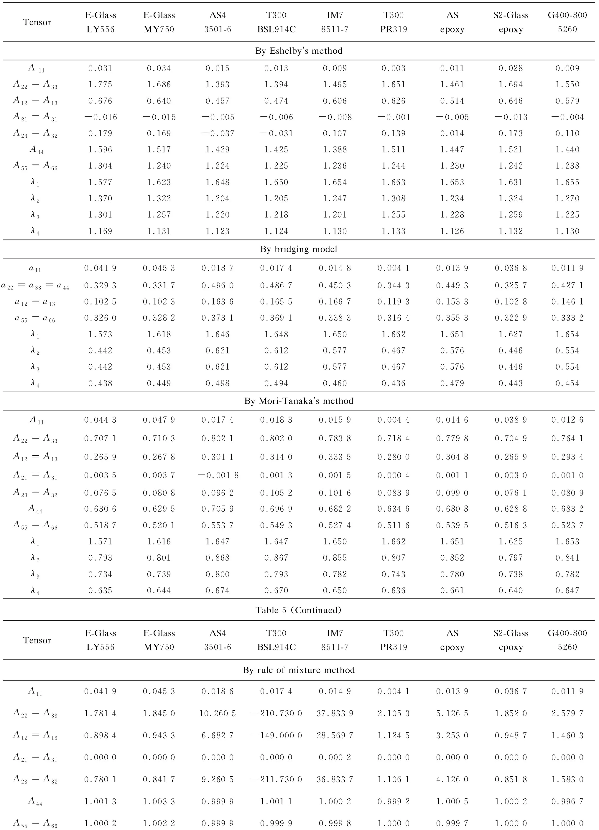
Table 5 Non-zero bridging tensor elements and coefficients λi’s for the 9 composites by different models

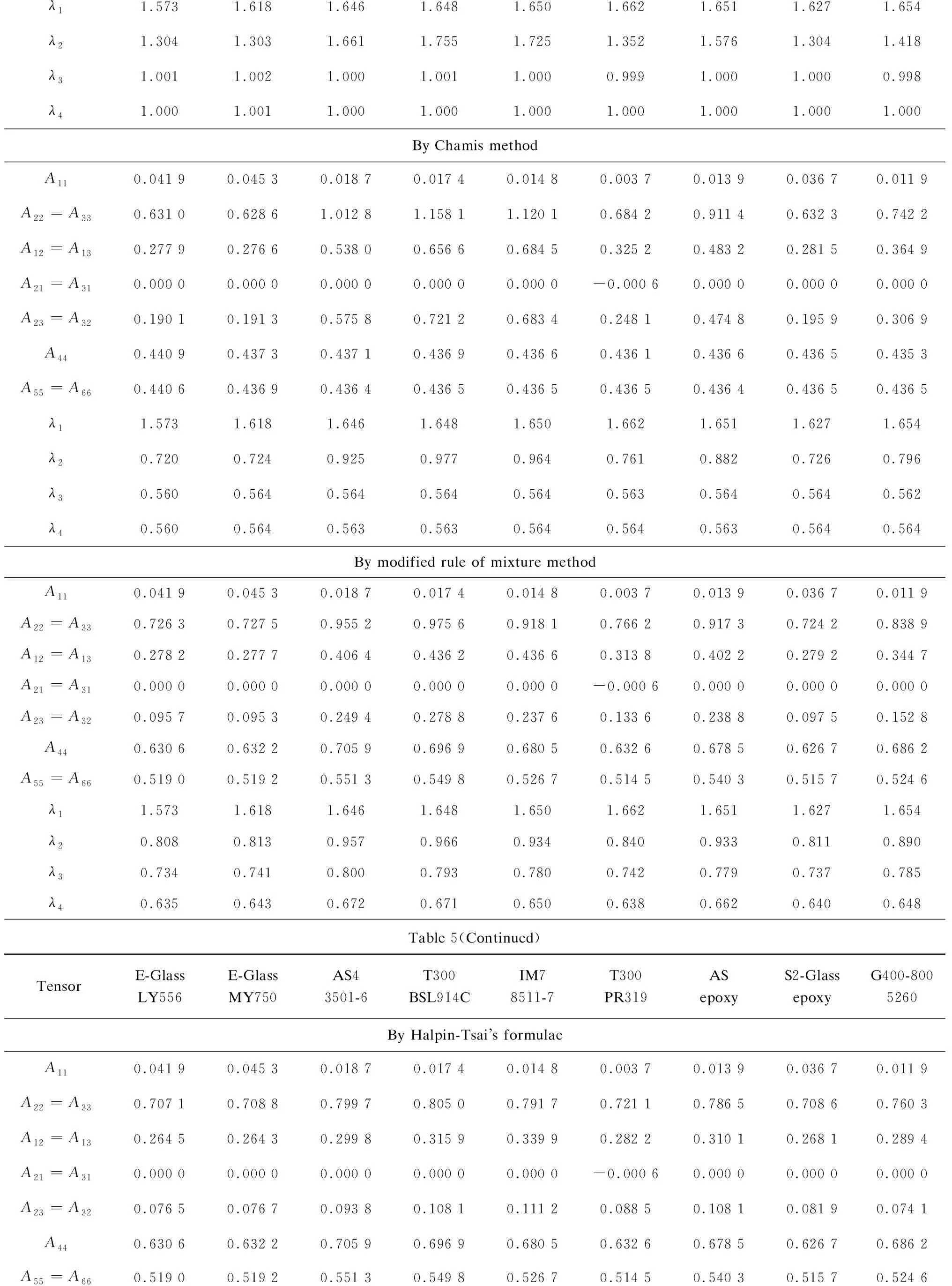
λ11.5731.6181.6461.6481.6501.6621.6511.6271.654 λ21.3041.3031.6611.7551.7251.3521.5761.3041.418 λ31.0011.0021.0001.0011.0000.9991.0001.0000.998 λ41.0001.0011.0001.0001.0001.0001.0001.0001.000 By Chamis methodA110.041 90.045 30.018 70.017 40.014 80.003 70.013 90.036 70.011 9 A22=A330.631 00.628 61.012 81.158 11.120 10.684 20.911 40.632 30.742 2 A12=A130.277 90.276 60.538 00.656 60.684 50.325 20.483 20.281 50.364 9 A21=A310.000 00.000 00.000 00.000 00.000 0-0.000 60.000 00.000 00.000 0 A23=A320.190 10.191 30.575 80.721 20.683 40.248 10.474 80.195 90.306 9 A440.440 90.437 30.437 10.436 90.436 60.436 10.436 60.436 50.435 3 A55=A660.440 60.436 90.436 40.436 50.436 50.436 50.436 40.436 50.436 5 λ11.5731.6181.6461.6481.6501.6621.6511.6271.654 λ20.7200.7240.9250.9770.9640.7610.8820.7260.796 λ30.5600.5640.5640.5640.5640.5630.5640.5640.562 λ40.5600.5640.5630.5630.5640.5640.5630.5640.564 By modified rule of mixture methodA110.041 90.045 30.018 70.017 40.014 80.003 70.013 90.036 70.011 9 A22=A330.726 30.727 50.955 20.975 60.918 10.766 20.917 30.724 20.838 9 A12=A130.278 20.277 70.406 40.436 20.436 60.313 80.402 20.279 20.344 7 A21=A310.000 00.000 00.000 00.000 00.000 0-0.000 60.000 00.000 00.000 0 A23=A320.095 70.095 30.249 40.278 80.237 60.133 60.238 80.097 50.152 8 A440.630 60.632 20.705 90.696 90.680 50.632 60.678 50.626 70.686 2 A55=A660.519 00.519 20.551 30.549 80.526 70.514 50.540 30.515 70.524 6 λ11.5731.6181.6461.6481.6501.6621.6511.6271.654 λ20.8080.8130.9570.9660.9340.8400.9330.8110.890 λ30.7340.7410.8000.7930.7800.7420.7790.7370.785 λ40.6350.6430.6720.6710.6500.6380.6620.6400.648 Table 5(Continued)TensorE-GlassLY556E-GlassMY750AS43501-6T300BSL914CIM78511-7T300PR319AS epoxyS2-GlassepoxyG400-8005260By Halpin-Tsai s formulaeA110.041 90.045 30.018 70.017 40.014 80.003 70.013 90.036 70.011 9 A22=A330.707 10.708 80.799 70.805 00.791 70.721 10.786 50.708 60.760 3 A12=A130.264 50.264 30.299 80.315 90.339 90.282 20.310 10.268 10.289 4 A21=A310.000 00.000 00.000 00.000 00.000 0-0.000 60.000 00.000 00.000 0 A23=A320.076 50.076 70.093 80.108 10.111 20.088 50.108 10.081 90.074 1 A440.630 60.632 20.705 90.696 90.680 50.632 60.678 50.626 70.686 2 A55=A660.519 00.519 20.551 30.549 80.526 70.514 50.540 30.515 70.524 6

λ11.5731.6181.6461.6481.6501.6621.6511.6271.654 λ20.7940.8000.8670.8700.8600.8090.8560.8000.839 λ30.7340.7410.8000.7930.7800.7420.7790.7370.785 λ40.6350.6430.6720.6710.6500.6380.6620.6400.648By Hill-Hashin-Christensen-Lo s methodA110.044 20.047 7-----0.039 4-A22=A330.628 80.658 6-----0.646 1-A12=A130.249 60.270 8-----0.265 9-A21=A310.003 40.003 7-----0.003 7-A23=A320.109 30.140 7-----0.134 1-A440.519 50.517 8-----0.512 1-A55=A660.519 00.519 2-----0.515 7-λ11.571 01.616 0-----1.625 0-λ20.7270.755-----0.745-λ30.6360.642-----0.636-λ40.6350.643-----0.640-By self-consistent methodA110.048 60.052 20.020 40.019 20.017 00.004 70.015 40.042 70.013 3 A22=A330.347 40.375 30.721 10.706 30.668 20.425 40.656 20.351 80.602 0 A12=A130.137 00.147 70.284 50.287 10.300 20.176 90.269 60.140 00.236 8 A21=A310.009 60.009 90.002 60.002 60.002 90.000 90.002 30.008 40.001 9 A23=A320.068 00.072 60.126 60.123 90.129 50.082 40.121 90.069 10.081 3 A440.279 50.302 70.594 50.582 40.538 80.343 10.534 30.282 60.520 7 A55=A660.132 20.147 90.281 60.270 90.183 40.099 10.234 70.127 10.166 4 λ11.5671.6121.6451.6461.6491.6621.6501.6221.653 λ20.4590.4960.8060.7950.7640.5490.7550.4710.713 λ30.3850.4200.7100.6990.6610.4650.6570.3960.644 λ40.1970.2240.3950.3820.2720.1550.3380.1950.250 Table 5(Continued)TensorE-GlassLY556E-GlassMY750AS43501-6T300BSL914CIM78511-7T300PR319AS epoxyS2-GlassepoxyG400-8005260By generalized self-consistent methodA110.044 30.047 70.019 60.018 30.015 20.004 50.014 60.039 40.012 6 A22=A330.704 80.708 30.804 40.802 00.783 70.721 80.787 30.706 60.761 0 A12=A130.264 20.266 00.303 20.314 00.333 90.283 10.310 90.267 70.290 1 A21=A310.003 50.003 70.001 30.001 30.000 60.000 50.001 10.003 70.001 0 A23=A320.074 20.077 50.098 50.105 20.103 20.089 30.108 90.078 60.074 8 A440.630 60.630 80.705 90.696 90.680 50.632 60.678 50.628 00.686 2 A55=A660.519 00.519 20.552 00.549 80.526 70.514 50.540 30.515 70.524 6 λ11.5711.6161.6461.6471.6501.6621.6511.6251.653

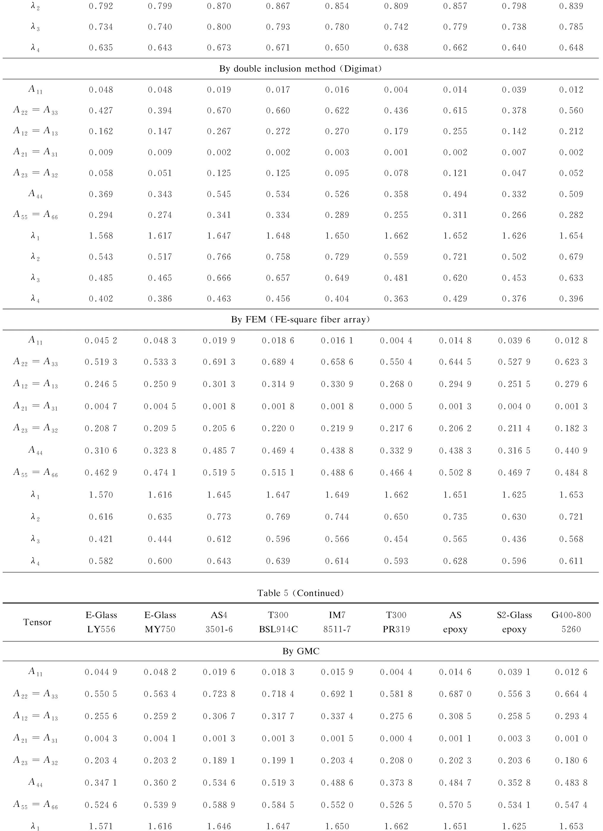
λ20.7920.7990.8700.8670.8540.8090.8570.7980.839 λ30.7340.7400.8000.7930.7800.7420.7790.7380.785 λ40.6350.6430.6730.6710.6500.6380.6620.6400.648 By double inclusion method (Digimat)A110.0480.0480.0190.0170.0160.0040.0140.0390.012A22=A330.4270.3940.6700.6600.6220.4360.6150.3780.560A12=A130.1620.1470.2670.2720.2700.1790.2550.1420.212A21=A310.0090.0090.0020.0020.0030.0010.0020.0070.002A23=A320.0580.0510.1250.1250.0950.0780.1210.0470.052A440.3690.3430.5450.5340.5260.3580.4940.3320.509A55=A660.2940.2740.3410.3340.2890.2550.3110.2660.282λ11.5681.6171.6471.6481.6501.6621.6521.6261.654λ20.5430.5170.7660.7580.7290.5590.7210.5020.679λ30.4850.4650.6660.6570.6490.4810.6200.4530.633λ40.4020.3860.4630.4560.4040.3630.4290.3760.396By FEM (FE-square fiber array)A110.045 20.048 30.019 90.018 60.016 10.004 40.014 80.039 60.012 8 A22=A330.519 30.533 30.691 30.689 40.658 60.550 40.644 50.527 90.623 3 A12=A130.246 50.250 90.301 30.314 90.330 90.268 00.294 90.251 50.279 6 A21=A310.004 70.004 50.001 80.001 80.001 80.000 50.001 30.004 00.001 3 A23=A320.208 70.209 50.205 60.220 00.219 90.217 60.206 20.211 40.182 3 A440.310 60.323 80.485 70.469 40.438 80.332 90.438 30.316 50.440 9 A55=A660.462 90.474 10.519 50.515 10.488 60.466 40.502 80.469 70.484 8 λ11.5701.6161.6451.6471.6491.6621.6511.6251.653 λ20.6160.6350.7730.7690.7440.6500.7350.6300.721 λ30.4210.4440.6120.5960.5660.4540.5650.4360.568 λ40.5820.6000.6430.6390.6140.5930.6280.5960.611 Table 5 (Continued)TensorE-GlassLY556E-GlassMY750AS43501-6T300BSL914CIM78511-7T300PR319AS epoxyS2-GlassepoxyG400-8005260By GMCA110.044 90.048 20.019 60.018 30.015 90.004 40.014 60.039 10.012 6 A22=A330.550 50.563 40.723 80.718 40.692 10.581 80.687 00.556 30.664 4 A12=A130.255 60.259 20.306 70.317 70.337 40.275 60.308 50.258 50.293 4 A21=A310.004 30.004 10.001 30.001 30.001 50.000 40.001 10.003 30.001 0 A23=A320.203 40.203 20.189 10.199 10.203 40.208 00.202 30.203 60.180 6 A440.347 10.360 20.534 60.519 30.488 60.373 80.484 70.352 80.483 8 A55=A660.524 60.539 90.588 90.584 50.552 00.526 50.570 50.534 10.547 4 λ11.5711.6161.6461.6471.6501.6621.6511.6251.653

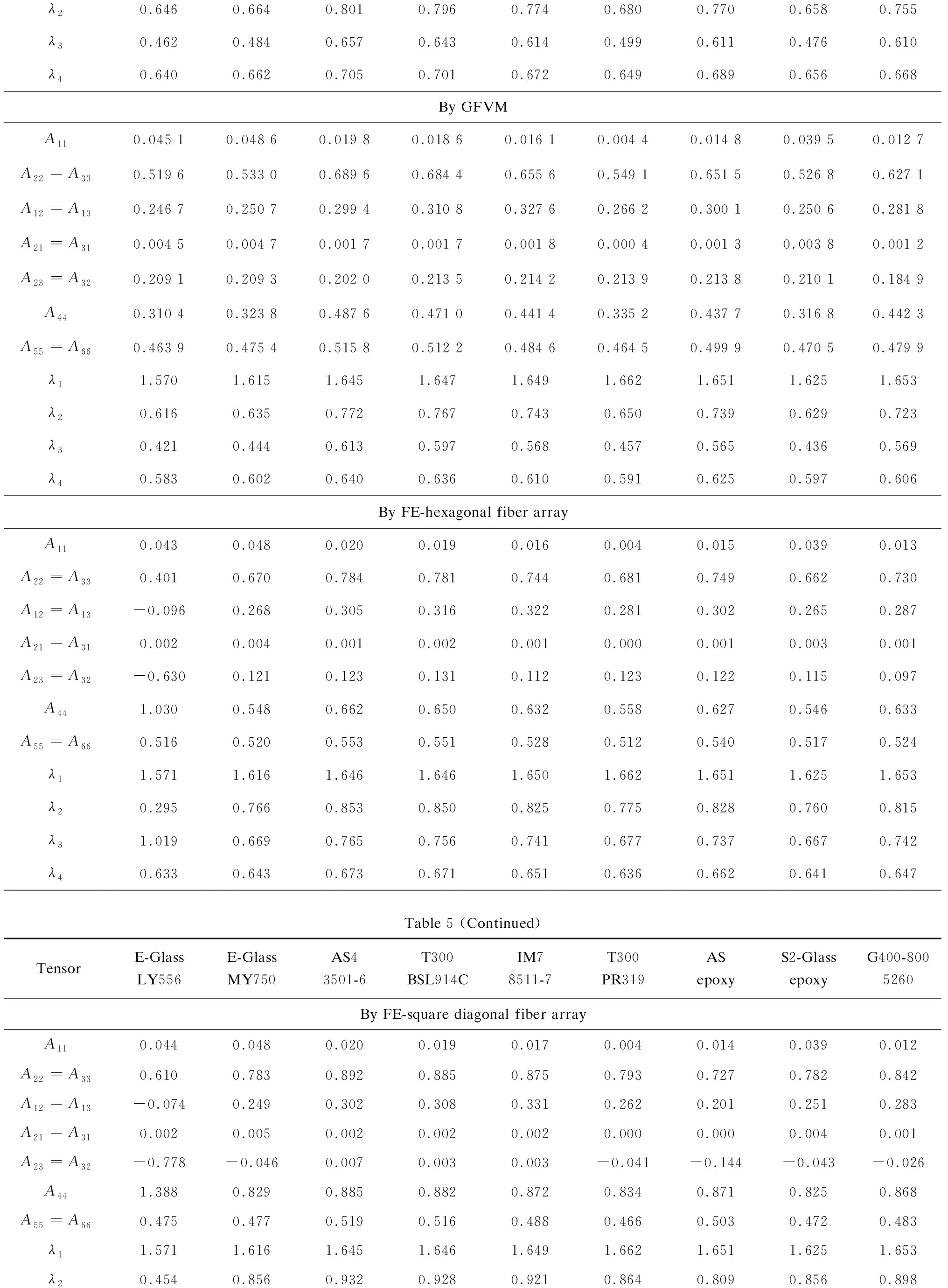
λ20.6460.6640.8010.7960.7740.6800.7700.6580.755 λ30.4620.4840.6570.6430.6140.4990.6110.4760.610 λ40.6400.6620.7050.7010.6720.6490.6890.6560.668 By GFVMA110.045 10.048 60.019 80.018 60.016 10.004 40.014 80.039 50.012 7 A22=A330.519 60.533 00.689 60.684 40.655 60.549 10.651 50.526 80.627 1 A12=A130.246 70.250 70.299 40.310 80.327 60.266 20.300 10.250 60.281 8 A21=A310.004 50.004 70.001 70.001 70.001 80.000 40.001 30.003 80.001 2 A23=A320.209 10.209 30.202 00.213 50.214 20.213 90.213 80.210 10.184 9 A440.310 40.323 80.487 60.471 00.441 40.335 20.437 70.316 80.442 3 A55=A660.463 90.475 40.515 80.512 20.484 60.464 50.499 90.470 50.479 9 λ11.5701.6151.6451.6471.6491.6621.6511.6251.653 λ20.6160.6350.7720.7670.7430.6500.7390.6290.723 λ30.4210.4440.6130.5970.5680.4570.5650.4360.569 λ40.5830.6020.6400.6360.6100.5910.6250.5970.606 By FE-hexagonal fiber arrayA110.0430.0480.0200.0190.0160.0040.0150.0390.013A22=A330.4010.6700.7840.7810.7440.6810.7490.6620.730A12=A13-0.0960.2680.3050.3160.3220.2810.3020.2650.287A21=A310.0020.0040.0010.0020.0010.0000.0010.0030.001A23=A32-0.6300.1210.1230.1310.1120.1230.1220.1150.097A441.0300.5480.6620.6500.6320.5580.6270.5460.633A55=A660.5160.5200.5530.5510.5280.5120.5400.5170.524λ11.5711.6161.6461.6461.6501.6621.6511.6251.653λ20.2950.7660.8530.8500.8250.7750.8280.7600.815λ31.0190.6690.7650.7560.7410.6770.7370.6670.742λ40.6330.6430.6730.6710.6510.6360.6620.6410.647Table 5 (Continued)TensorE-GlassLY556E-GlassMY750AS43501-6T300BSL914CIM78511-7T300PR319AS epoxyS2-GlassepoxyG400-8005260By FE-square diagonal fiber arrayA110.0440.0480.0200.0190.0170.0040.0140.0390.012A22=A330.6100.7830.8920.8850.8750.7930.7270.7820.842A12=A13-0.0740.2490.3020.3080.3310.2620.2010.2510.283A21=A310.0020.0050.0020.0020.0020.0000.0000.0040.001A23=A32-0.778-0.0460.0070.0030.003-0.041-0.144-0.043-0.026A441.3880.8290.8850.8820.8720.8340.8710.8250.868A55=A660.4750.4770.5190.5160.4880.4660.5030.4720.483λ11.5711.6161.6451.6461.6491.6621.6511.6251.653λ20.4540.8560.9320.9280.9210.8640.8090.8560.898

λ31.2100.8900.9280.9260.9190.8930.9180.8870.916λ40.5940.6040.6430.6400.6130.5930.6280.5990.609By FE-random fiber arrayA110.0470.0500.0210.0200.0170.0050.0150.0410.013A22=A330.6030.6220.9011.4300.8560.6470.8450.5950.749A12=A130.2580.2700.3990.8130.4290.2900.3890.2550.321A21=A310.0070.0070.0040.0040.0030.0010.0020.0060.002A23=A320.1550.1710.2810.8900.2780.1820.2710.1530.174A440.4470.4510.6200.5400.5780.4660.5740.4420.576A55=A660.5220.5250.5810.5540.5700.5140.5610.5200.536λ11.5701.6151.6451.6471.6491.6621.6511.6251.653λ20.6600.6760.8300.8260.8020.6940.7980.6620.777λ30.5660.5780.7310.6620.6950.5920.6920.5690.693λ40.6110.6210.6060.6010.6340.6090.6500.6150.629

Using the relevant parameters in Tables 1 and 2, the SCFs of the matrix in each of the 9 composites are calculated, as indicated in Table 6. The predicted strengths are compared with the experimental measurements (Table 2), and the averaged relative correlation errors for all of the 14 models are summarized in Table 7. Bridging Model is still overall the most accurate, although the accuracy difference between the Bridging Model’s and the other models’ predictions for the strengths is less than those for the elastic properties of the composites. As more than double of the constituent data and more other information are required, meaning that more than double the accumulated error may be involved, a reasonable correlation error to be expected in a micromechanical strength prediction would be greater than 10% and up to 20%. Table 7 shows that this is attainable by the current theory.

Table 6 SCFs of the matrices in the 9 composites

Table7Overallaveragederrorsinpredictionoftheuniaxialstrengthsofthe9UDcompositesbydifferentmicromechanicsmodels

ModelNAveraged error*(%)Error ratioRankBridging model5321.11.001Double inclusion (Digimat)5321.91.042GFVM5323.01.093FE-square5323.11.094Chamis model5325.41.205GMC5325.41.205FE-random5328.51.306Hill-Hashin-C-L model1830.11.437Halpin-Tsai formulae5330.11.437Generalized self-consistent5330.21.438Mori-Tanaka method5330.21.438Modified rule of mixture5330.71.459FE-square diagonal5331.91.5110FE-hexagonal5332.01.5211Self consistent method5332.71.5412Rule of mixture method5344.52.1113Eshelby s method5345.12.1414

8 Consistency

A necessary and sufficient condition for a micromechanics model to be consistent is that its bridging tensor is always in an upper triangular form. If, for instance,A320, we will get from Eq. (2) that0 and from Eq. (3) that0, where [Bij]=(Vf[I]+Vm[Aij])-1. The bridging tensor of Bridging Model, by definition, is always upper triangular, even when the matrix of a constituent undergoes a plastic deformation[16]. On the other hand, Table 5 shows that all of the other models are not consistent. The non-consistency implies that the homogenized internal stresses should be calculated using the full 3D stress formulae, even though the composite is subjected to a uniaxial load. To apply an analytical model other than Bridging Model to the stress calculation, the 3D compliance tensors of the fiber, matrix and the composite should be used in Eq. (5) to obtain the 3D bridging tensor. If a numerical method is applied to predict a composite property, a 3D rather than 2D RVE geometry should be discretized.

9 Conclusion

Once SCFs of the matrix in a composite are determined and are taken into account, any micromechanics model originally developed for composite stiffness can perform a reasonable prediction for a composite strength as well. An assessment on the predictive ability of 14 models for the stiffness and strength of a UD composite against the benchmark data in WWFEs indicates that Bridging Model operates with the smallest correlation error in both the stiffness and strength predictions. Moreover, it is the only consistent model in the internal stress calculation. A full 3D approach should be applied if any other model is used to simulate a composite’s effective property.

Acknowledgements

We greatly appreciate the help of Dr. Chen at Xi’an Jiaotong University for supplying the data in Table 3 predicted by finite volume method and generalized method of cells.