STABILITY OF TRAVELING WAVES IN A POPULATION DYNAMIC MODEL WITH DELAY AND QUIESCENT STAGE∗
2018-07-23YonghuiZHOU周永辉YunruiYANG杨赟瑞KepanLIU刘克盼
Yonghui ZHOU(周永辉)Yunrui YANG(杨赟瑞) Kepan LIU(刘克盼)
School of Mathematics and Physics,Lanzhou Jiaotong University,Lanzhou 730070,China
E-mail:1169524175@qq.com;lily1979101@163.com;sophialiu16@163.com
Abstract This article is concerned with a population dynamic model with delay and quiescent stage.By using the weighted-energy method combining continuation method,the exponential stability of traveling waves of the model under non-quasi-monotonicity conditions is established.Particularly,the requirement for initial perturbation is weaker and it is uniformly bounded only at x=+∞but may not be vanishing.
Key words Stability;traveling waves;weighted-energy method
1 Introduction
Many practical problems we meet in biology,chemistry,epidemiology,and population dynamics[1,17]are often described by reaction-diffusion scalar equations and systems.For example,the following reaction-diffusion system
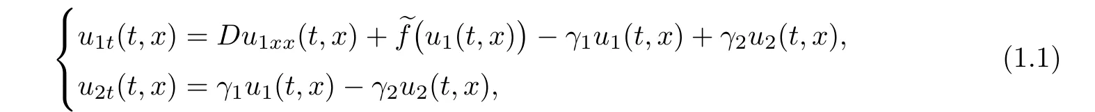
which represents a population dynamic model with a quiescent stage where individuals migrate and reproduce are subject to randomly occurring inactive phases,where u1and u2denote the densities of mobile and stationary subpopulations,respectively.D>0 is the diffusion coefficient of the mobile subpopulation,is the reproduction function,γ1>0 is the rate of switching from a mobile state to stationary state,and γ2>0 is the rate of switching from a stationary state to mobile state.For more details about this model,one can refer to[4,5].
Considering the fact that growth rate of the population is instantaneous whereas there may be a time delay that should be taken into account,such as the duration of maturation,gestation and hatching period and so on,the following reaction-diffusion system with delay is more truthful,where τ≥0 is the delay.A special case of system(1.2)is the diffusive Nicholson’s blow flies equation with a quiescent stage and delay

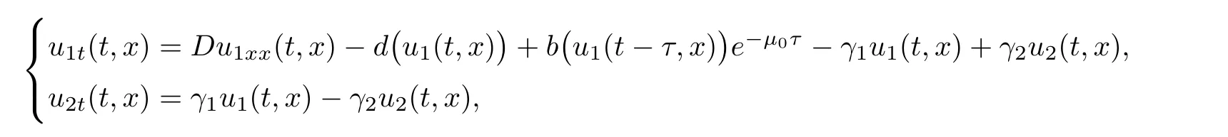
where u1(t,x)and u2(t,x)are the densities of mobile and stationary subpopulations of the mature blow flies at time t and a point x,respectively,b(·)is the birth rate of the mature,d(·)is the death of the mature,µ0is the death rate of the juvenile,and the delay τ≥ 0 is the duration of the juvenile state.
Because of their important role in the above fields mentioned,traveling wave solutions of reaction-diffusion equations with(or without)delay were extensively investigated and there were many important results;see[1–3,9–16,18,19].For example,some existence results on traveling wave solutions of(1.1)and(1.2)were attained.In 2007,Zhang and Zhao[22]obtained the existence of spreading speed for(1.1)and showed that it coincides with the minimal wave speed for monotone traveling wave solutions.After that,Zhang and Li[23]considered the monotonicity and uniqueness of traveling wave solutions of(1.1).Recently,using comparison arguments,Schauder’s fixed point theorem,and a limit process,Zhao and Liu[24]established the existence of spreading speed of(1.2)and characterized it as the minimal wave speed for traveling wave solutions in non-quasi-monotone case.In addition,the stability of traveling waves is always one of the important and difficult objects in the traveling waves theory.For the monotone case,the frequently used methods are squeezing technique,weighted energy method combining comparison principle,convergence theory for monotone semi flows,and spectral analysis method.For example,using the weighted energy method combining comparison principle motivated by Mei’s idea[9,14,15]for scalar equations,Yang[20]established the globally exponential stability of monotone traveling wave solutions for an epidemic system with delay,which extended the results for scalar equations to systems.
However,for the non-monotone case,the stability results of traveling waves are limited,because comparison principle does not still hold and it is difficult to establish the spectral analysis for delayed systems without quasi-monotonicity.Fortunately,the weighted-energy method combining continuation method developed by Mei[12,13]is an effective way to solve the stability of traveling waves for nonmonotone equations,and it does not need comparison principle to hold.In 2013,Yang and Li et al[21] first generalized the kind of weighted-energy method to an epidemic system with delay and without quasi-monotonicity and established the stability of traveling waves.After that,Lin and Mei et al[10]proved the exponential stability of traveling waves,which can be either monotone or nonmonotone with any speed c>c∗and any size of the time-delay by using the weighted energy method combining continuation method.They improved the previous results in[12,13]because they restrict the initial perturbation only inwith a uniform bound but not be vanishing as x→+∞,which differs from the previous works where the weight function are selected to be greater than 1 for all x and the initial perturbation must converge to 0 in.Motivated by Lin’s idea[10],the purpose of this article is to establish the stability of nonmonotone traveling waves of system(1.2)by the weighted energy method.It generalizes the result of scalar equation with delay in Lin’s[10]to system with delay and improves the previous results in[21]by the weaker requirement for initial perturbation.
The rest of this article is organized as follows.In Section 2,we introduce some preliminaries and state our stability result.In Section 3,we prove our main result on the exponential stability of traveling waves.
2 Preliminaries and Main Result
NotationsThroughout this article,C>0 denotes a generic constant,Ci>0(i=1,2,···)represents a specific constant.Let I be an interval.L2(I)is the space of the square integrable functions defined on I,and Hk(I)(k≥0)is the Sobolev space of the L2-function h(x)defined on the interval I whose derivatives(i=1,2,···,k)also belong to L2(I).denotes the weighted L2-space with a weight function w(x)>0 and its norm is defined byis the weighted Sobolev space with the norm given by

Let T>0 be a number and B be a Banach space.C([0,T];B)is the space of B-valued continuous functions on[0,T].L2([0,T];B)is the space of B-valued L2-functions on[0,T].The corresponding spaces of B-valued functions on[0,∞)are defined similarly.
Moreover,we need the following assumptions for the sake of the existence of traveling wave solutions(see[24]):
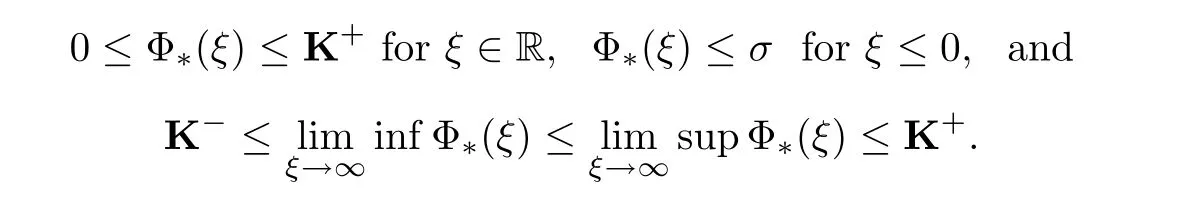
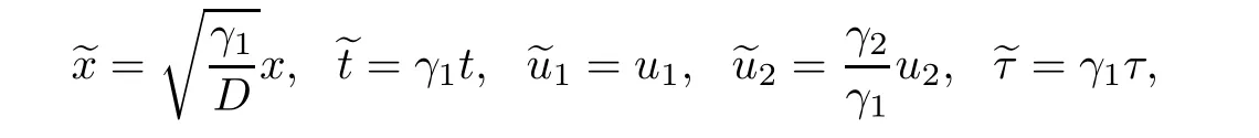
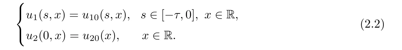
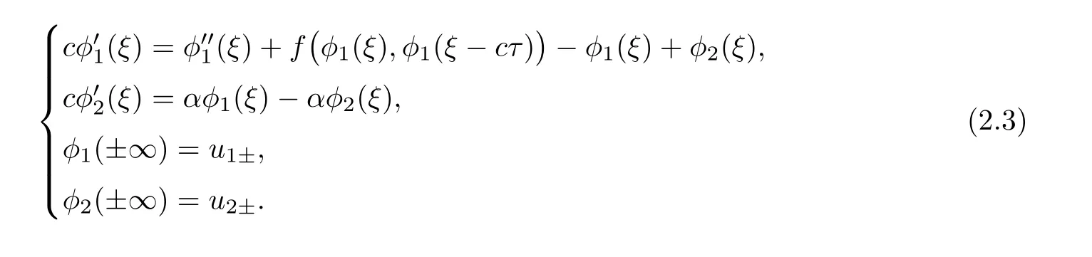
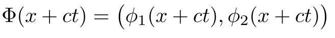
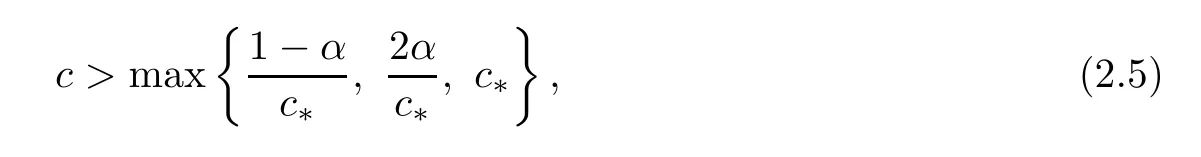
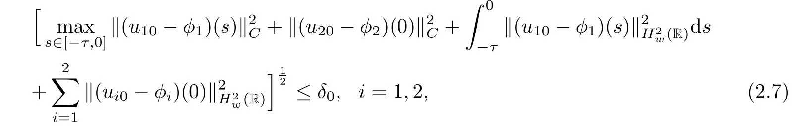
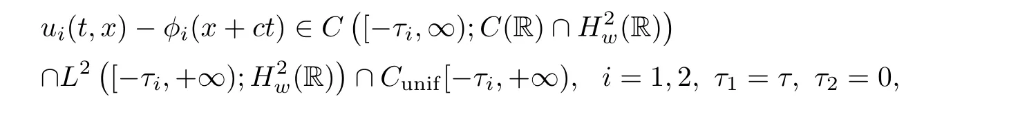
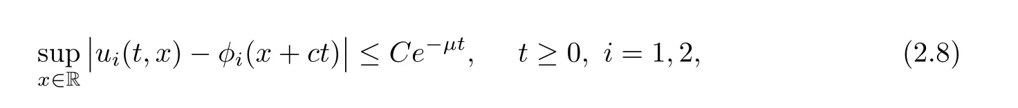
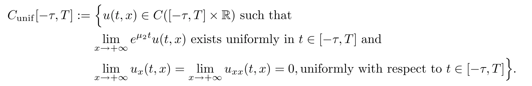
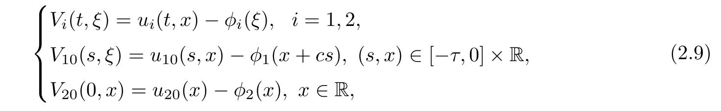
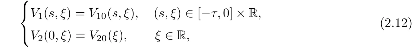
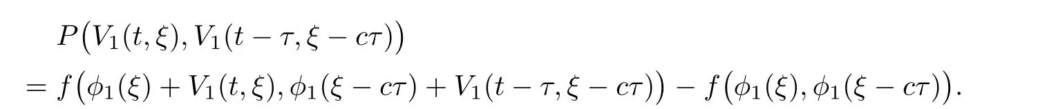
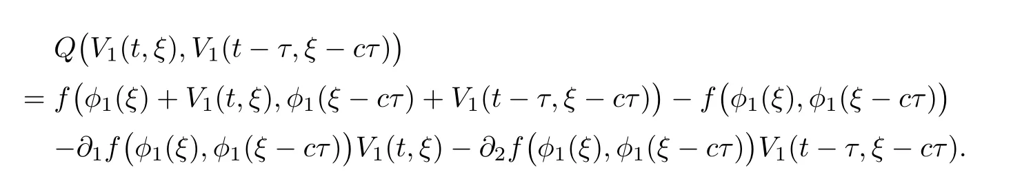
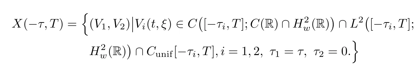
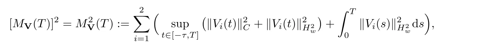
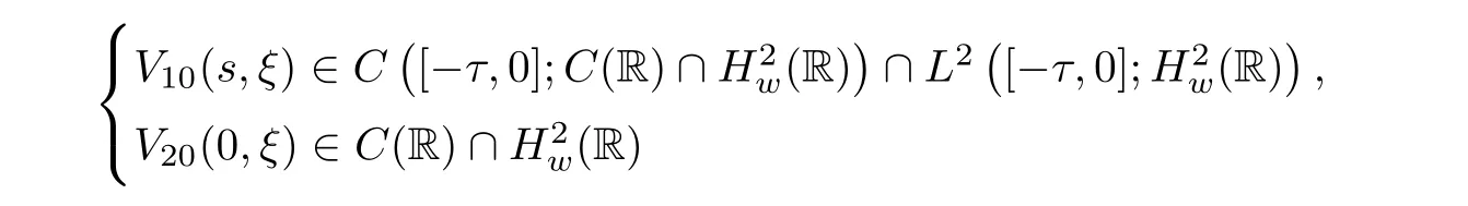
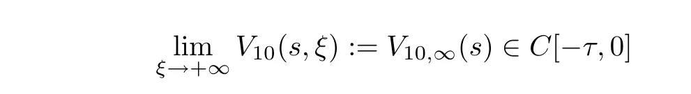
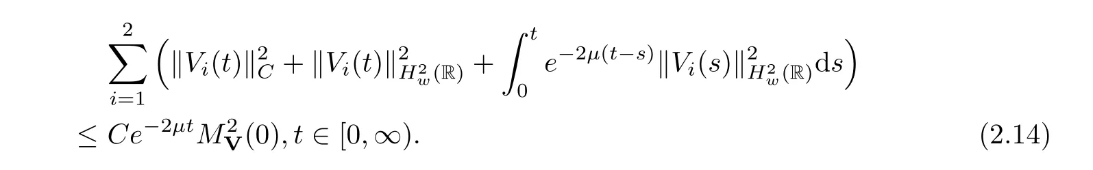
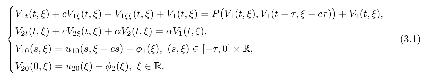
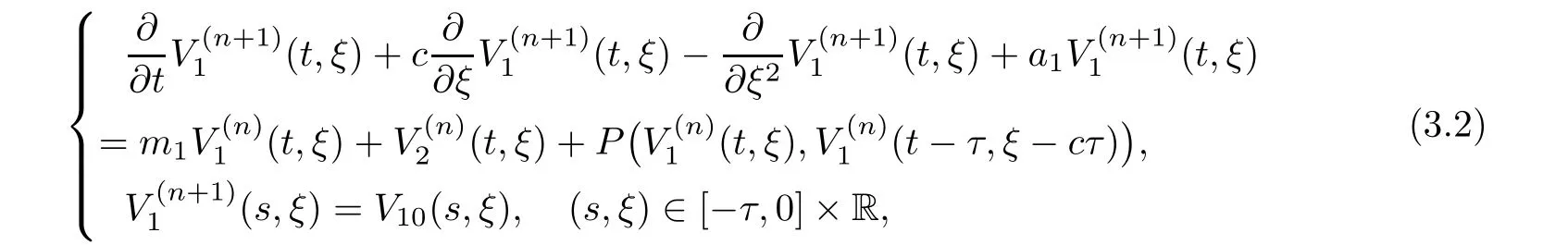
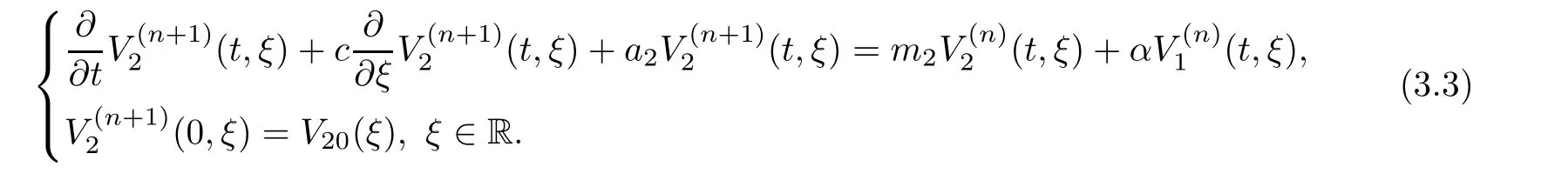
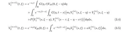
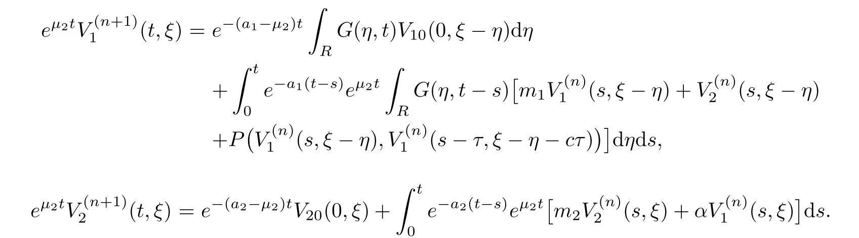
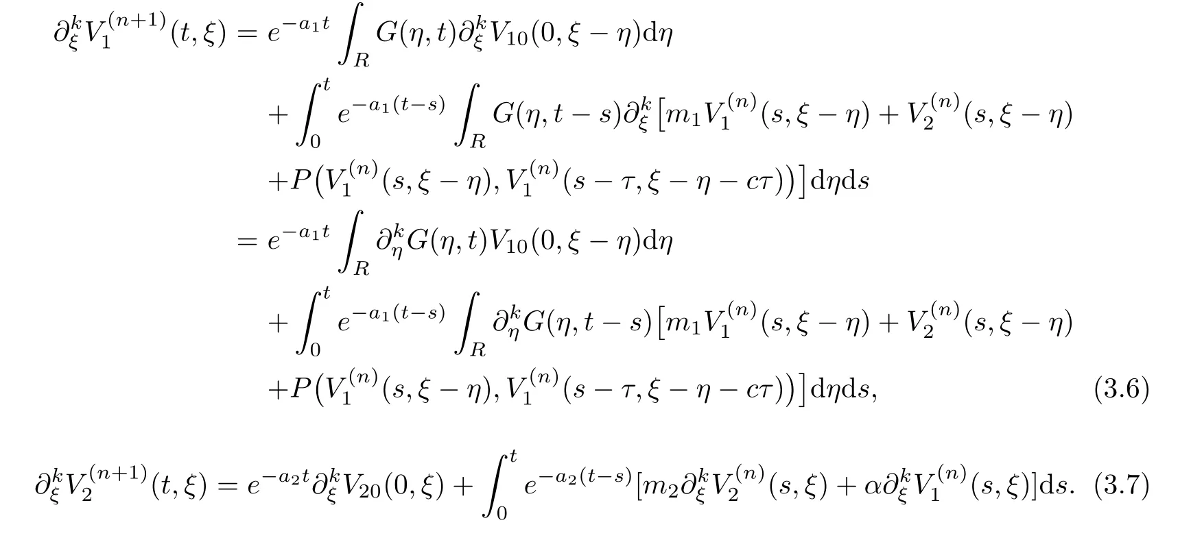
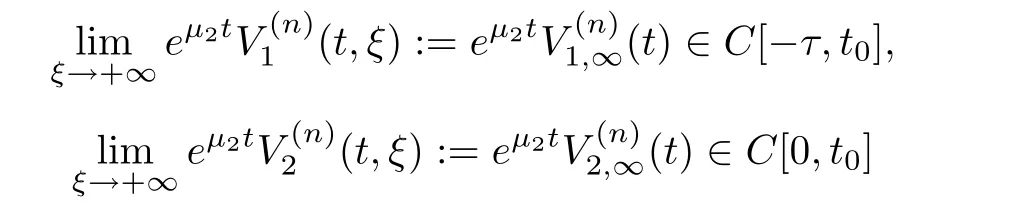
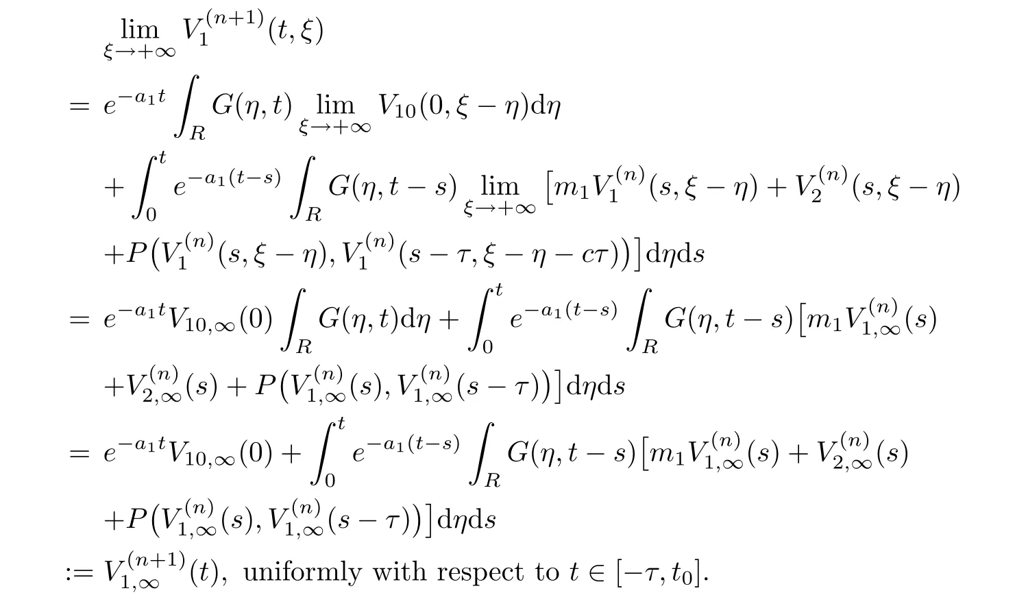
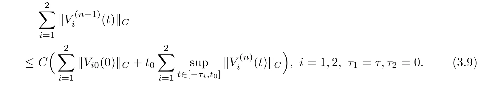
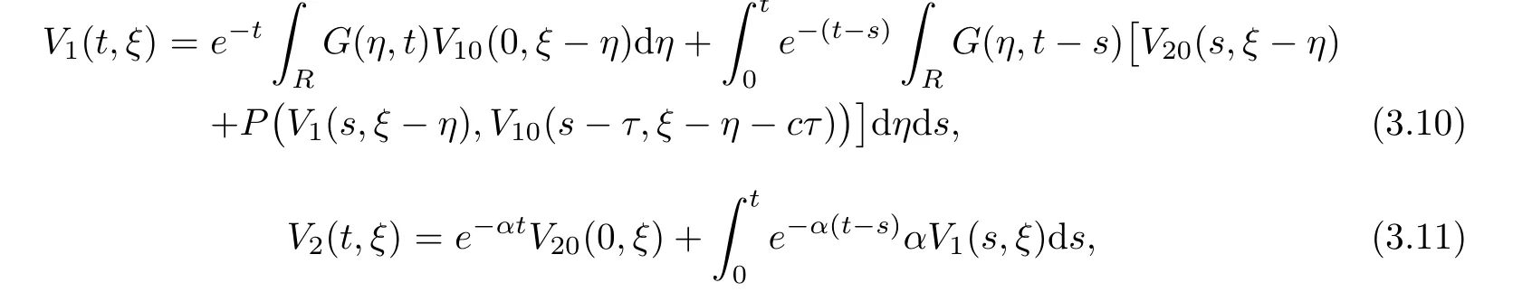
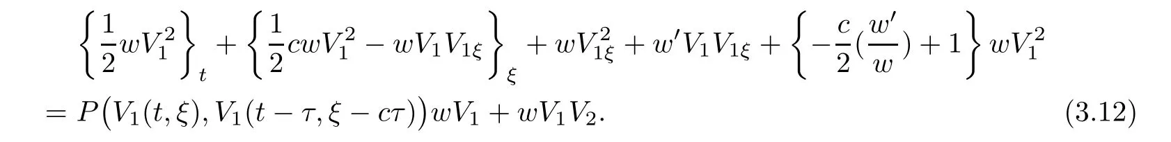
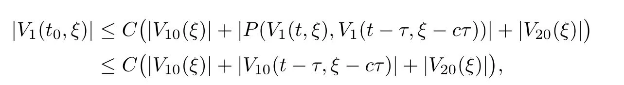
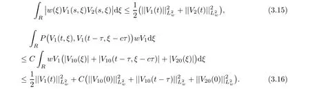
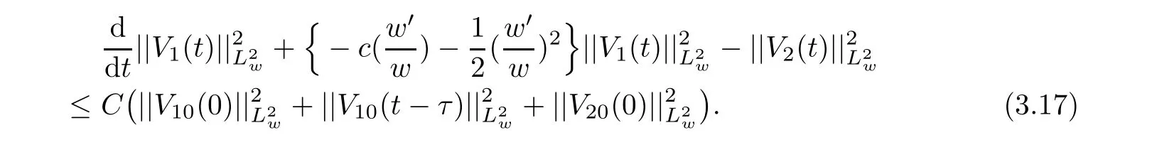
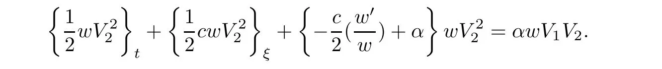
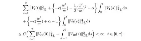
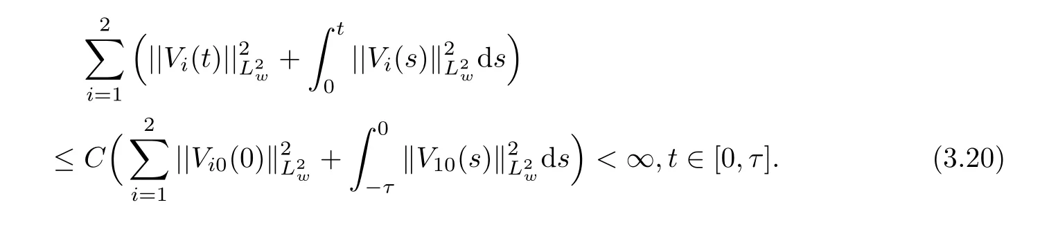
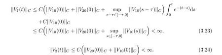
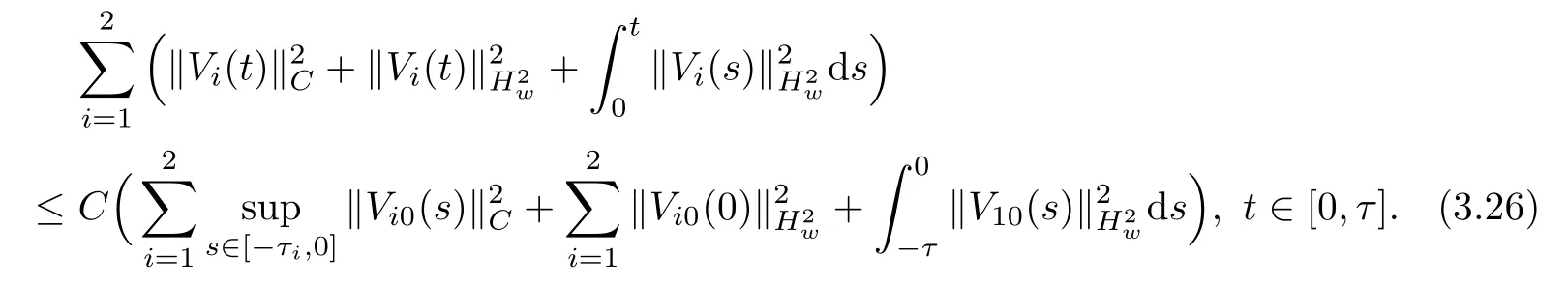
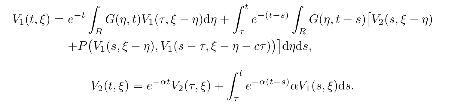
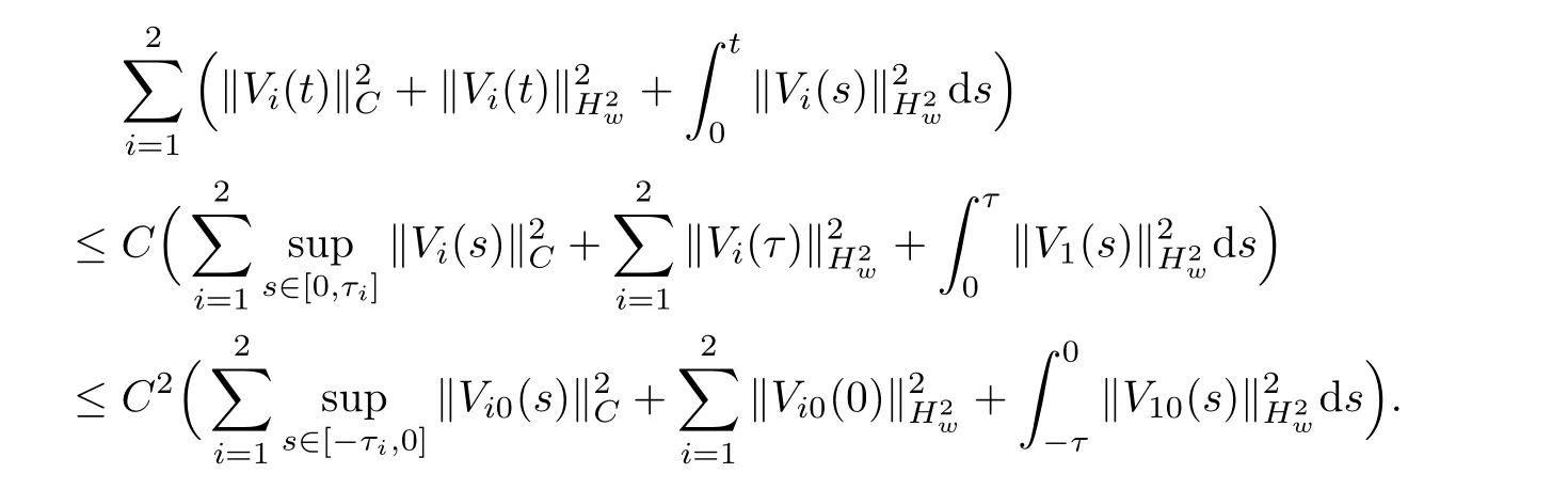
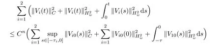
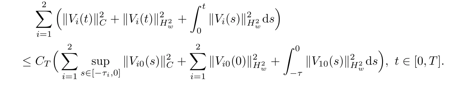
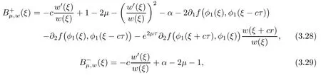
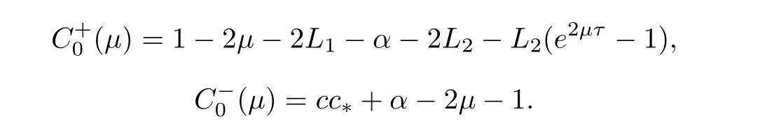
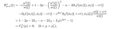
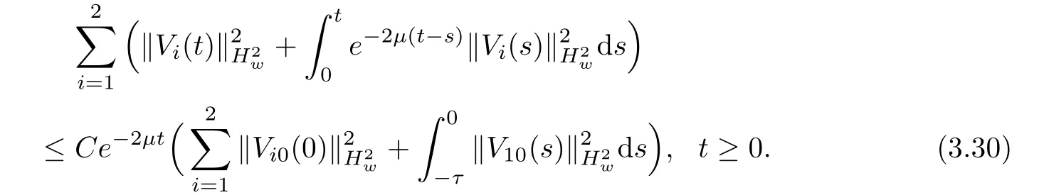
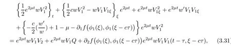
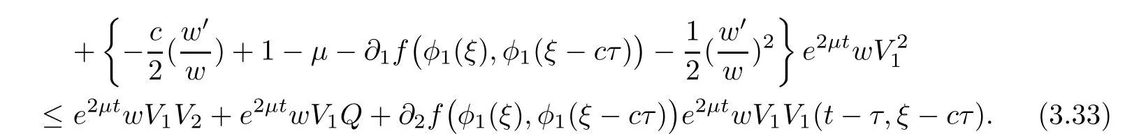
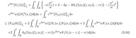
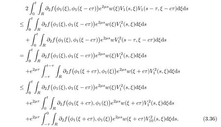
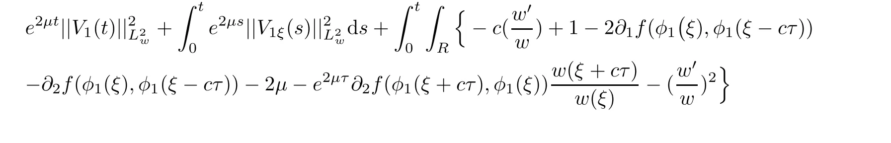
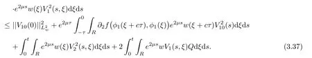
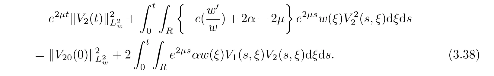
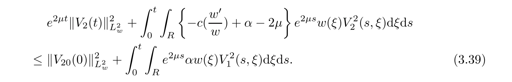
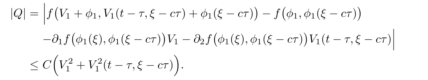
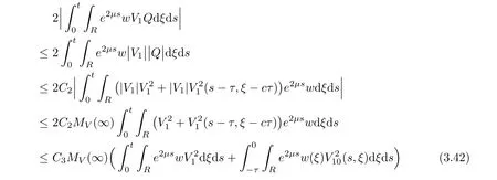
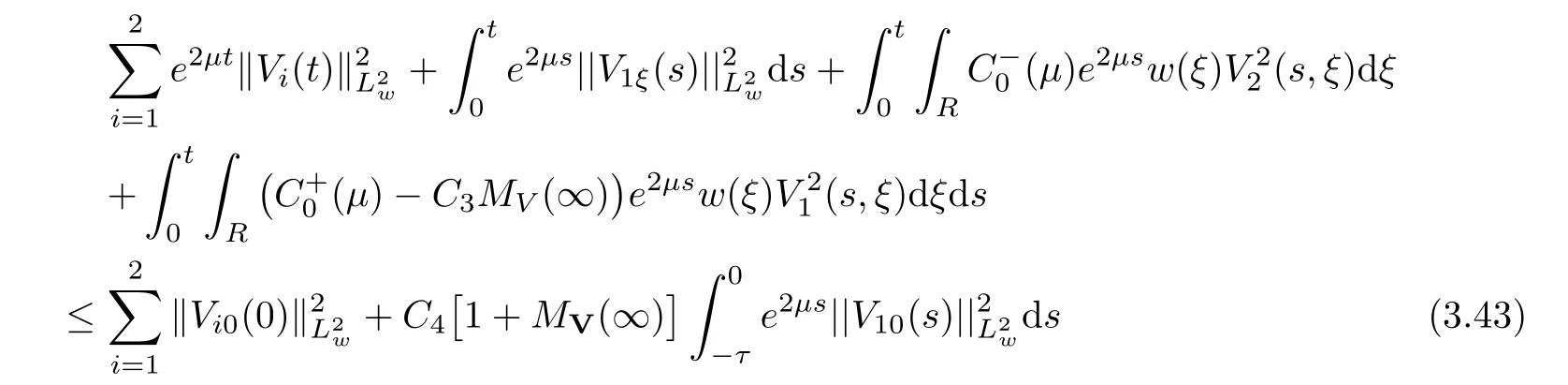
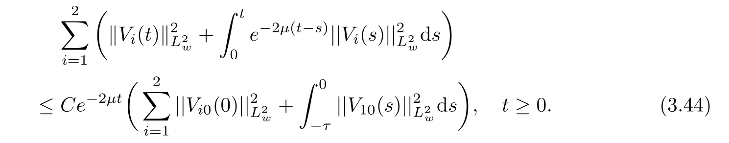
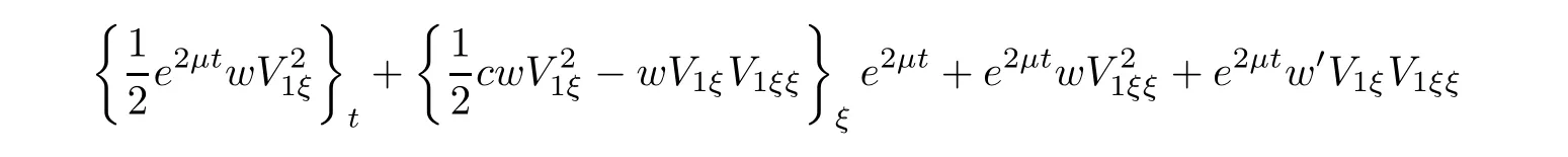
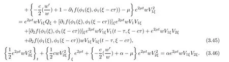
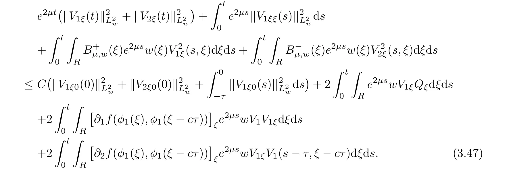
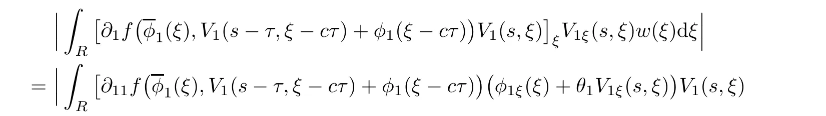
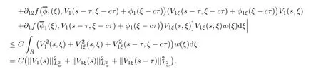
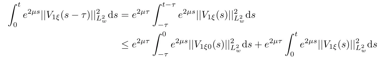
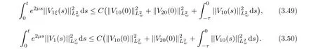
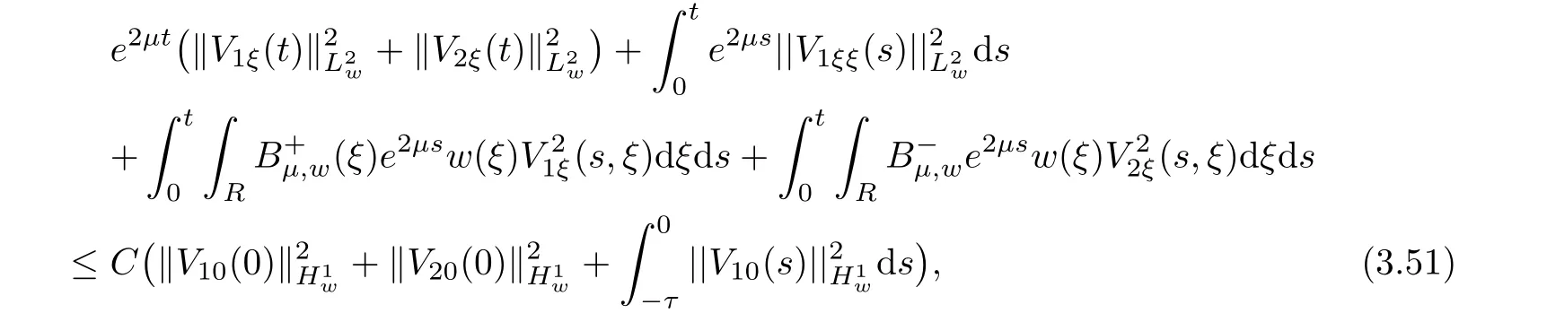
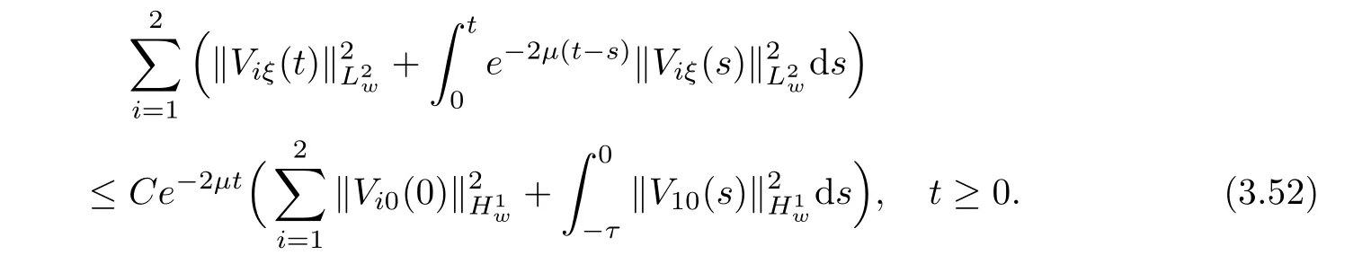
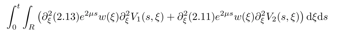
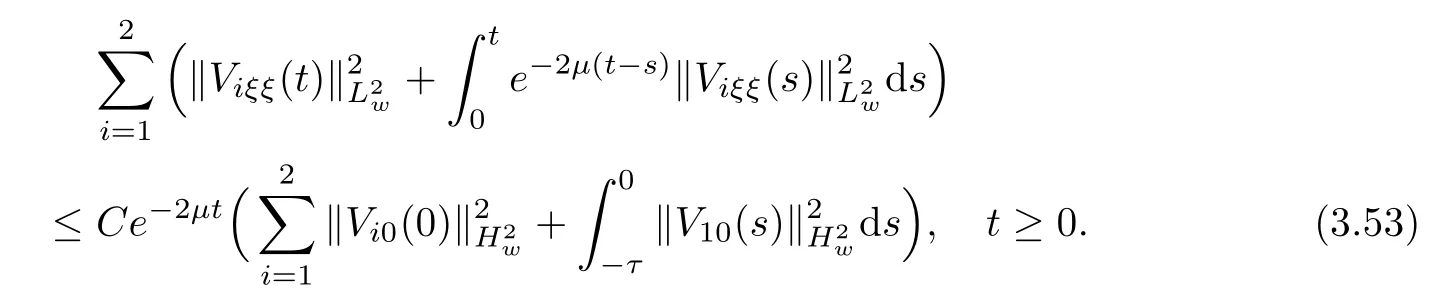
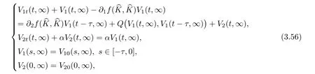
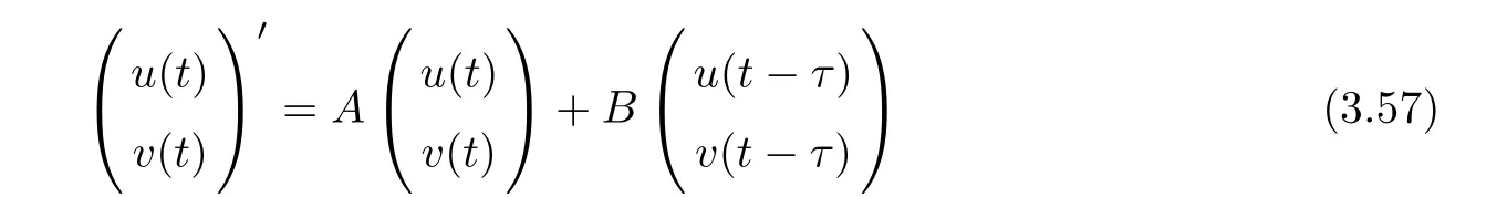
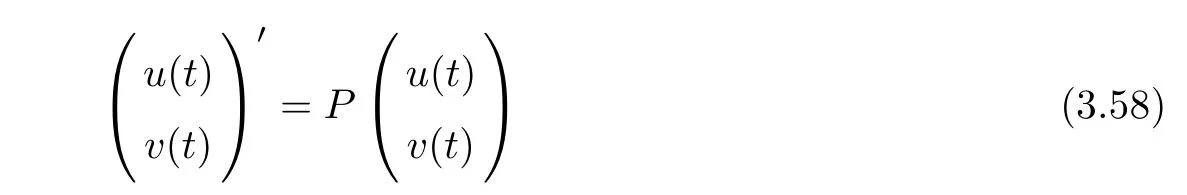
(A1)There exist K±and K>0 with 0 (A2)for u1,u2∈ [0,K],where α0>0 is a constant and g(·)is a given function,g(u)/u is strictly decreasing for u∈[K−,K+]andsatisfies the property: (P)∀u1,u2∈[K−,K+]satisfying u2≤K≤u1,u2≥b(u1)and u1≤b(u2),there holds u1=u2. Notice that system(1.2)has two constant equilibria u−=(u1−,u2−)=(0,0)and u+=(u1+,u2+)=(K,K0),whereand K,K0>0.Zhao[24]proved the existence of traveling wave solutions of(1.2)with pro fileby the idea of auxiliary equations and Schauder’s fixed-point theorem. Proposition 2.1(Existence of traveling waves) Assume that(A1)holds.Then,there exists c∗>0 such that Moreover,if(A2)holds,then (ii) for c=c∗,for any vector σ ≫ 0 with||σ||≪ 1,(1.2)admits a non-constant traveling wave solution Φ∗(ξ)such that Moreover,Φ∗(−∞)=0 and if(A2)holds,then (iii)for 0 Mathematically,for simplification,letting that is,scaling the spatial,time variables,and absorbing the appropriate constant into u1in(1.2),in this article,it suffices to study the following system(dropping the tildes on x,t,u1,u2,τ for notational convenience) The existence of traveling wave solutions of(2.1)is guaranteed by Proposition 2.1.Because the rescaling is made,we denote the two constant equilibria of(2.1)as u−=(0,0)andwhereWe are interested in traveling wave solutions of(2.1)that connect u−with u+.A traveling wave solution of system(2.1)connecting with u−and u+is a solution(here the notation of traveling waves is still used byand is not distinguished)satisfying the following ordinary differential system For some kind of need for proof,we denote Define a weight function as where c∗is the speed of critical waves and is defined by Proposition 2.1. Next,we state our main result about the exponential stability of traveling wave solutions of(2.1). we obtain the following fact: If the initial perturbation satisfies then,the solution(u1(t,x),u2(t,x))of the Cauchy problem(2.1)and(2.2)is unique,exists globally in time,and satisfies and where Cunif[−τ,T],for τ≥ 0,0 Remark 2.3The results of scalar equations with delay in[10,11]are generalized to system with delay and without quasi-monotonicity in this article. Remark 2.4The previous results in[12,13,21]are improved by the weaker requirement for initial perturbation,which is different from the previous work.Here,the initial perturbation is allowed being uniformly bounded only at x=+∞but may not be disappearing,namely, The proof is similar to Yang[21],so we omit it here. then,initial problem(2.1)and(2.2)can be reformulated as with the initial conditions where where Define and where τ1= τ, τ2=0,T>0.Therefore,Theorem 2.2 is equivalent to the following result. and exists uniformly with respect to s ∈ [−τ,0],where w(ξ)is the weighted function given in(2.4),then,there exist positive constants δ0and µ such that,when MV(0) ≤δ0,the solutionof the Cauchy problem(2.10)–(2.12)uniquely and globally exists in X(−τ,∞),and satisfies To investigate the stability of traveling wave solutions of(2.1),we need to establish the global existence and uniqueness result of solution for the perturbed system and a prior estimate.We first prove the following local existence result of solutions,which will be used later. Proposition 3.1(Local estimate) Consider the following Cauchy problem ProofThe proof is trivial by the standard iteration technique and thus it is omitted here.In contrast to previous works,here,we only need to show that the local solution V∈for some small t0>0 will be determined later.The proof is motivated by that of Lin[10][Proposition 2.2]and we sketch the proof as follows. and Therefore,(3.2)and(3.3)can be written in the integral form Moreover, In fact,by the facts that the uniform boundedness of Therefore, On the other hand, Therefore,we have Furthermore,by taking the regular energy estimate we can estimate From(3.4)and(3.5),we get Combining(3.8)and(3.9),we prove ProofThe proof is mainly motivated by that of[16].When t∈ [0,τ],(2.10)–(2.12)with the initial data(V10(s,ξ),V20(0,ξ))∈ X(−τ,0)can be uniquely solved as By Taylor’s formula,it is not difficult to verify that holds in[0,t0]for some small constant t0>0.For t ∈ [t0,2t0],again by Taylor’s formula,it holds that From(3.10), with 0≤t≤t0.Then,it holds that for t∈ [t0,2t0].Repeating the step in each of the intervals[nt0,(n+1)t0],n=1,2,3,···,one by one,then(3.14)holds for all t∈ [0,τ].Using Cauchy-Schwarz inequality again,we have Substituting(3.15)and(3.16)into(3.13),we get Integrating(3.17)with respect to t∈ [0,τ]over[0,t],we obtain Multiplying(2.11)by w(ξ)V2(t,ξ),we get Integrating the above equality over R × [0,t]with respect to ξ and t,we further obtain Combining(3.18)and(3.19),we have Thus,by(2.5),we obtain Furthermore,differentiating(2.10)–(2.11)with respect to ξ and multiplying the resultant equations by w(ξ)V1ξ(t,ξ)and w(ξ)V2ξ(t,ξ),respectively,by the same arguments as above,we obtain Similarly,we have For t∈ [0,τ],from(3.10)–(3.11),we obtain Combining(3.23)and(3.24),we obtain When t ∈ [τ,2τ],the solutions of(2.10)–(2.12)with the initial data(V1(s,ξ),V2(s,ξ)) ∈Xloc(0,τ)can be uniquely solved as By the same arguments as(3.12)–(3.26),we can prove(V1,V2) ∈ Xloc(τ,2τ),and when t ∈[τ,2τ],we have Repeating the above procedure,step by step,thenuniquely exists,and satisfies for t∈ [(n−1)τ,nτ],and we can prove that(V1,V2)is unique and(V1,V2)∈ Xloc(−τ,∞)with,for any T>0,that Proposition 3.3(A prior estimate) Letbe a local solution of the Cauchy problem(2.11)–(2.13).Then,there exist positive constants µ and δ2independent of a given constant T>0 such that,when MV(0)≤ δ2, Define and In the followings,we prove Proposition 3.3 by a series of lemmas. Lemma 3.4(Key inequality) Let w(ξ)be the weight function given in(2.4).If(2.5)holds,then ProofFirst of all,we proveholds.From(2.4),we have w(ξ)=Note thatThus,we obtain This completes the proof. Lemma 3.5LetThen,there exist positive constants µ1and δ2such that,when 0< µ < µ1and MV(∞)≤ δ2,it holds that ProofWe prove estimate(3.30)in three steps. Step 1The estimate for Vi(t,ξ)in,i=1,2. Multiplying(2.13)and(2.11)by e2µtw(ξ)V1(t,ξ)and e2µtw(ξ)V2(t,ξ),respectively,we obtain and By the Cauchy-Schwarz inequality,(3.31)is reduced to Integrating(3.33)over R × [0,t]with respect to ξ and t,it follows that For the second term of the right side in(3.34),using the Cauchy-Schwarz inequality again,we can estimate that Similarly,we can estimate that Substituting(3.35)and(3.36)into(3.34),and using w(ξ)≥ 0,0 ≤ φ1(ξ)≤ K,and µ ∈ (0,µ1),we have On the other hand,integrating(3.32)over R × [0,t]with respect to ξ and t,we have Using the Cauchy-Schwarz inequality,we obtain Therefore,(3.38)is reduced to Combining(3.37)and(3.39),we get Next,we are going to estimate the nonlinear term on the right-hand side of(3.41).By Taylor’s formula,we have By the standard Sobolev embedding inequality H1(R)ô→ C(R)and the modified embedding inequalityas w(ξ)>0 defined in(2.4),for t>0, ξ∈ R,we have for some positive constant C4=max{C1,C3}>0. Let MV(∞) ≪ 1,becausefor 0< µ < µ1,we can find a positive constant δ2>0 such that.When,we obtainThen,it follows that Step 2The estimate for Viξ(t,ξ)in Similarly,by differentiating(2.13)and(2.11)with respect to ξ,and multiplying the resultant equations by e2µtw(ξ)V1ξ(t,ξ)and e2µtw(ξ)V2ξ(t,ξ),respectively,we get Integrating(3.45)and(3.46)over R × [0,t]with respect to ξ and t,by similar arguments as above,we obtain Now,we estimate the last three terms of the right-hand side in(3.47), Next,we estimate the first term of right side in(3.48).Noting that V1(s,ξ)and φ1(ξ)are bounded by some constants and using the condition(A1),we obtain The other terms of right side in(3.48)can be estimated similarly;hence,for the last three terms in(3.47),we have It is also noted that and it follows from(3.43)that Substituting(3.49)and(3.50)into(3.47),we obtain Therefore,for i=1,2,it holds that Step 3The estimate forin Similarly,by taking and using the results in Step 1 and Step 2,for i=1,2,it holds that Next,we establish the following Sobolev inequality. Lemma 3.6Letthen,it is equivalent toand and The proof is similar to Li[8],so we omit it here. Furthermore,the time-exponential decay of Vi(t,ξ)at ξ=+∞,i=1,2 is necessary.By the definition of Cunif[−τi,∞),it is obtained thatexists uniformly with respect to t∈ [−τi,∞),anduniformly with respect to t∈ [−τi,∞).Taking ξ→ +∞ to(2.13)and(2.11),we have with with the initial data ψ(s)and P=A+B.It is obvious that|λI − P|=0 if and only if and hence,it is easy to see that all the eigenvalues of the matrix P have negative real parts. Lemma 3.7Let X(t)be the solution of(3.56).Then,there exist positive constants τ0,µ2,such that,when τ< τ0, The proof of Lemma 3.7 is similar to Li[8];so we omit it here too. Now,as a nonlinear perturbation to linear delay system(3.57),by Lemma 3.7 and[6,Corollary 9.2.2],(3.56)satisfies the following nonlinear stability. Lemma 3.8Let(V1(t,∞),V2(t,∞))be the solution of(3.56).If τ< τ0,then, provided MV(0)≪ 1,where τ0, µ2>0 are defined in Lemma 3.7. Moreover,for i=1,2,because of uniformly in t ∈ [0,∞),namely,for any given positive number ε>0,there exists a positive number ξ0= ξ0(ε)sufficiently large and independent of t such that when ξ≥ ξ0, which implies that Let ε=MV(0),then we can get the following lemma. Lemma 3.9If τ< τ0,then,there exists a large number ξ0≫ 1(independent of t)such that Next,we prove Proposition 3.3. ProofBy Lemma 3.5,Lemma 3.6,and Lemma 3.9,we have This completes the proof. Finally,Theorem 2.6 is immediately followed from Proposition 3.2 and Proposition 3.3.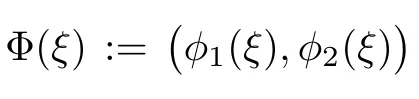


3 Proof of Main Result


杂志排行

Acta Mathematica Scientia(English Series)的其它文章
- GLOBAL EXISTENCE OF CLASSICAL SOLUTIONS TO THE HYPERBOLIC GEOMETRY FLOW WITH TIME-DEPENDENT DISSIPATION∗
- NONNEGATIVITY OF SOLUTIONS OF NONLINEAR FRACTIONAL DIFFERENTIAL-ALGEBRAIC EQUATIONS∗
- GROWTH AND DISTORTION THEOREMS FOR ALMOST STARLIKE MAPPINGS OFCOMPLEX ORDER λ∗
- EXACT SOLUTIONS FOR THE CAUCHY PROBLEM TO THE 3D SPHERICALLY SYMMETRIC INCOMPRESSIBLE NAVIER-STOKES EQUATIONS∗
- PRODUCTS OF RESOLVENTS AND MULTIVALUED HYBRID MAPPINGS IN CAT(0)SPACES∗
- CONVERGENCE FROM AN ELECTROMAGNETIC FLUID SYSTEM TO THE FULL COMPRESSIBLE MHD EQUATIONS∗