GLOBAL EXISTENCE OF CLASSICAL SOLUTIONS TO THE HYPERBOLIC GEOMETRY FLOW WITH TIME-DEPENDENT DISSIPATION∗

Dexing KONG(孔德兴)

School of Mathematical Sciences,Zhejiang University,Hangzhou 310027,China

E-mail:dkong@zju.edu.cn

Qi LIU(刘琦)†

Department of Applied Mathematics,College of Science,Zhongyuan University of Technology,Zhengzhou 450007,China

E-mail:21106052@zju.edu.cn

Abstract In this article,we investigate the hyperbolic geometry flow with time-dependent dissipation on Riemann surface.On the basis of the energy method,for 0<λ≤1,µ>λ+1,we show that there exists a global solution gijto the hyperbolic geometry flow with time-dependent dissipation with asymptotic flat initial Riemann surfaces.Moreover,we prove that the scalar curvature R(t,x)of the solution metric gijremains uniformly bounded.

Key words Hyperbolic geometry flow;time-dependent damping;classical solution;energy method;global existence

1 Introduction

Let M be an n-dimensional complete manifold with Riemannian metric gij.The following general version of hyperbolic geometry flow

was introduced by Kong and Liu in[4],where Rijis the Ricci curvature tensor of metric gijand Fijare some smooth functions of g andThe most important three cases are so-called standard hyperbolic geometry flow[5,6],the Einstein’s hyperbolic geometry flow[8],and the dissipative hyperbolic geometry flow[1,10].

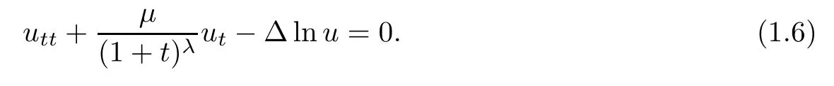
In this article,we are concerned with the hyperbolic geometry flow with time-dependent dissipation

with the initial metric on a Riemann surface

where u0(x1,x2)>0 is a smooth function.

In fact,on a surface,the metric can always be written(at least locally)in the following form

where u(t,x1,x2)>0 is a smooth function.Therefore,we have

Thus,equation(1.2)becomes

Denote

then,equation(1.6)becomes

Forµ=0,(1.2)is the standard hyperbolic geometry flow.In this case,Kong,Liu,and Xu[6]investigate the solution of equation(1.2)in one space dimension.They prove that the solution can exist for all time by choosing a suitable initial velocity.On the other hand,if the initial velocity tensor does not satisfy the condition presented in[6],the solution blows up at a finite time.Later,Kong,Liu,and Wang[5]consider the Cauchy problem for the hyperbolic geometry flow in two space variables with asymptotic flat initial Riemann surfaces,and give a lower bound of the life-span of classical solutions to the hyperbolic geometry flow.

Forµ>0,λ=0,(1.2)is the dissipative hyperbolic geometry flow.Liu[10]studies the solution of equation(1.2)in one space dimension and gains the similar results with Kong,Liu,and Xu[6].Kong,Liu,and Song[7]shown(1.2)that admits a global existence and established the asymptotic behavior of classical solutions to the dissipative hyperbolic geometry flow in two space variables.

Forµ >0 and λ >0,it is natural to ask:does the smooth solution of(1.2)blows up in finite time or does it exist globally?

In this article,we are interested in the hyperbolic geometry flow(1.2)with time-dependent dissipation in two space variables,that is,we consider the Cauchy problem for equation(1.8)with the following initial data

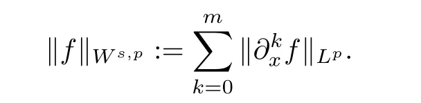
Throughout this article,we denote the general constants by C.[1,+∞],denotes the usual Sobolev space with its norm

We also always denote∂k= ∂xkand ∂kl= ∂xkxl.

The main results of this article can be described as follows.

Theorem 1.1Let 0< λ ≤ 1 and µ > λ+1.Suppose thatandis sufficiently small.Then,there exists a unique,global,classical solution of(1.8)–(1.9)satisfying

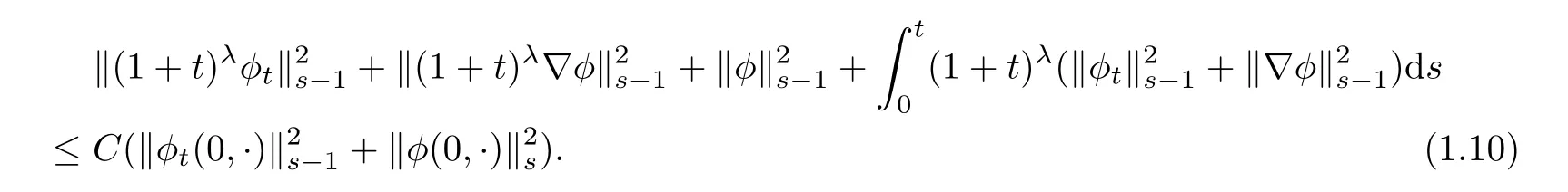
Theorem 1.2Under the assumptions mentioned in Theorem 1.1,the Cauchy problem(1.8)-(1.9)has a unique classical solution for all time;moreover,the scalar curvature R(t,x)corresponding to the solution metric gijremains uniformly bounded,that is,

where M is a positive constant,depending on the Hsnorm of φ0(x)and the Hs−1norm of φ1(x),but independent of t and x.

Remark 1.3Our main result,Theorem 1.1,gives a global existence of the classical solution of Cauchy problem(1.8)–(1.9).The theorem shows that,under suitable assumptions,the smooth evolution of asymptotic flat initial Riemann surfaces under the dissipative flow(1.2)exists globally on[0,+∞).

Remark 1.4Our main result,Theorem 1.1,gives a global existence of the classical solution of Cauchy problem(1.8)–(1.9)for 0< λ ≤ 1,µ> λ+1,while for the case 0<λ ≤ 1,µ≤λ+1,we have no idea to prove the global existence or blow up of the classical solution of the Cauchy problem.This implies that the relatively “large” dissipation has contribution to existence of the global solution,but for the relatively “small” dissipation,it is still unknown.

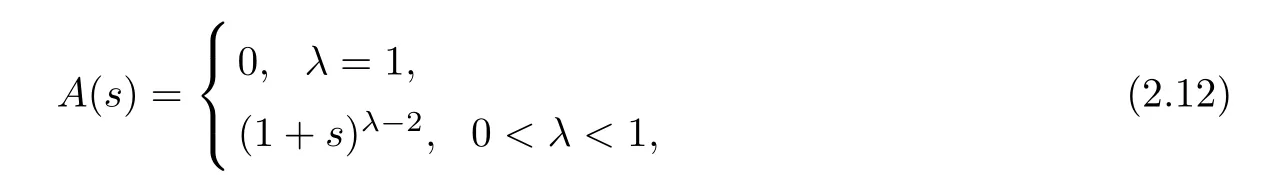
Set s≥4.Define

Moreover,we assume that for any t≥0,

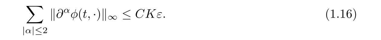
where K>0 is a suitably large constant.By Sobolev inequality,we have

Because(1.8)implies

we have

Let us indicate the proofs of Theorem 1.1.As in[2,11],in the following sections,we will eventually show thatwhenis assumed for some suitably large constant K>0 and small ε>0.Based on this and a continuous induction argument,the global existence of φ and then the main Theorem 1.1 are established for 0<λ≤1,µ>λ+1.

The rest of the article is arranged as follows.In Section 2,we will obtain the elementary estimate to the solution of(1.8)by using energy method.In Section 3,the estimates to higher derivatives will be considered,under which we show the global existence to the solution of the Cauchy problem(1.8)–(1.9),and prove the boundness of scalar curvature R(t,x)corresponding to the solution metric,that is,Theorem 1.1 and Theorem 1.2.

2 Elementary Energy Estimates

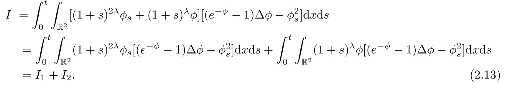
The equation(1.8)can be rewritten as

On one hand,multiplying(2.1)by m(1+t)2λφt,we have

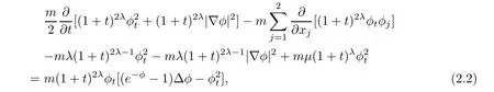
where m>0 will be determined later.Integrating it over R2×[0,t]yields

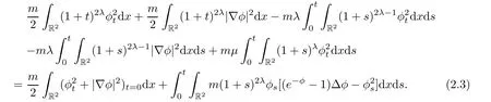
On the other hand,multiplying(2.1)by(1+t)λφ,we have

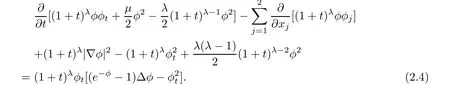
Integrating it over R2×[0,t]yields

For λ=1,combining(2.3)and(2.5),we obtain

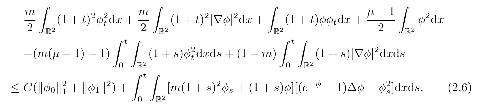
As µ >2,then letµ =2+4δ,where δ>0.Using Cauchy-Schwartz inequality,we have

in the left hand of(2.6)are all positive.Therefore,

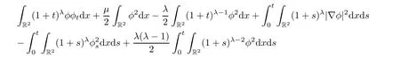
For 0<λ<1,combining(2.3)and(2.5),we obtain

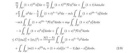
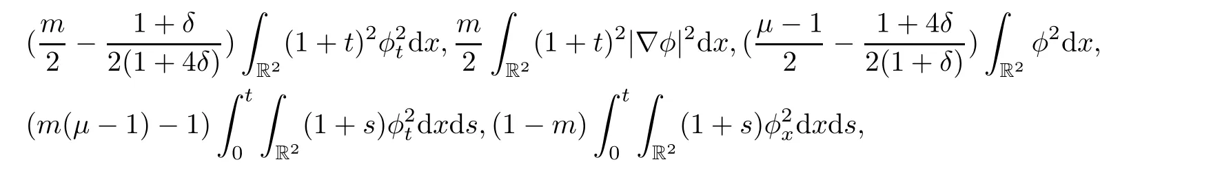
Becauseµ > λ+1,then letµ = λ+1+4δ,where δ>0.Using inequality(2.7),and choosingit is easy to show that the coefficients in the left hand of(2.9)are all positive.Therefore,

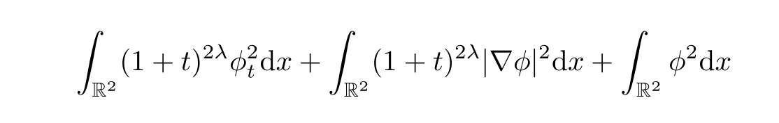
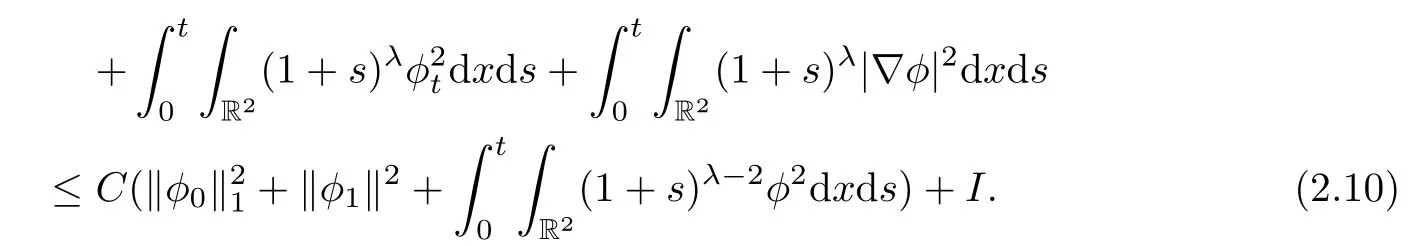
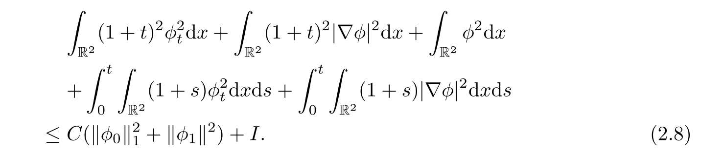
It follows from(2.8)and(2.10)that

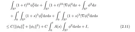
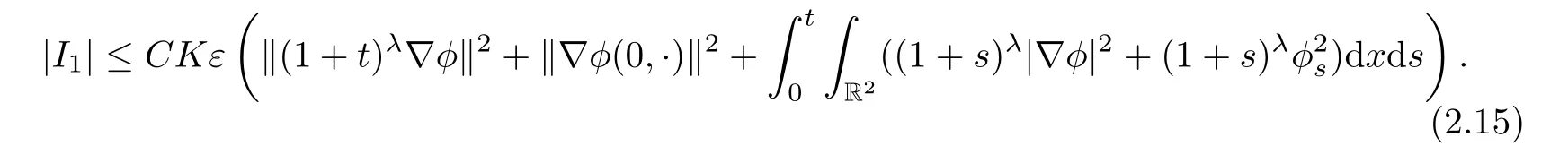
where

and

Because

thus,

Now,we consider I2.

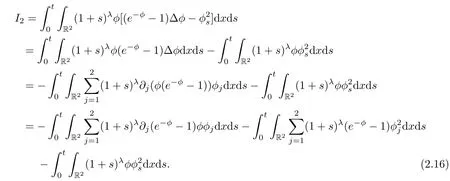
Thus,

By combining the above estimates,we get

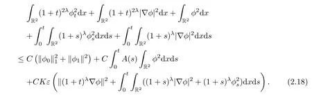
Thus,

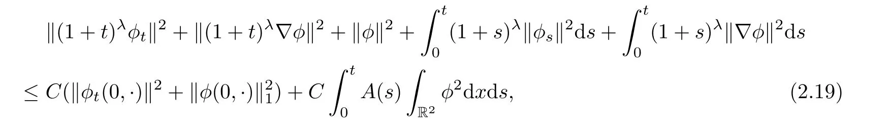
provided ε small enough.

3 Estimates on Higher Derivatives

The estimate as(2.19)can also be obtained for higher derivatives.In fact,by multiplying(2.1)bywe have

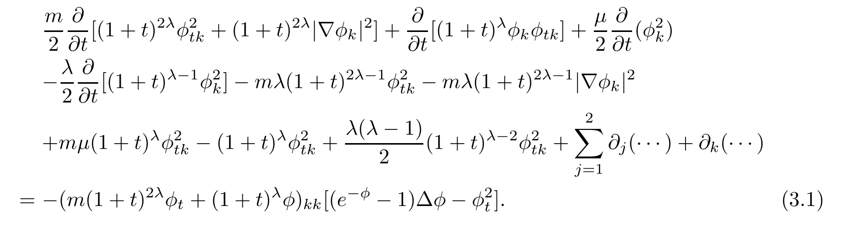
Integrating it over R2×[0,t]yields

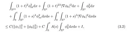
where

Because

we have the followings:

First

thus,

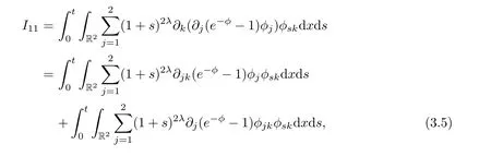
Next,we consider I12,

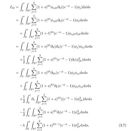
thus,

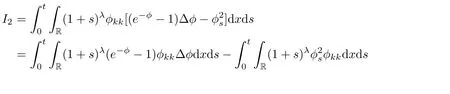
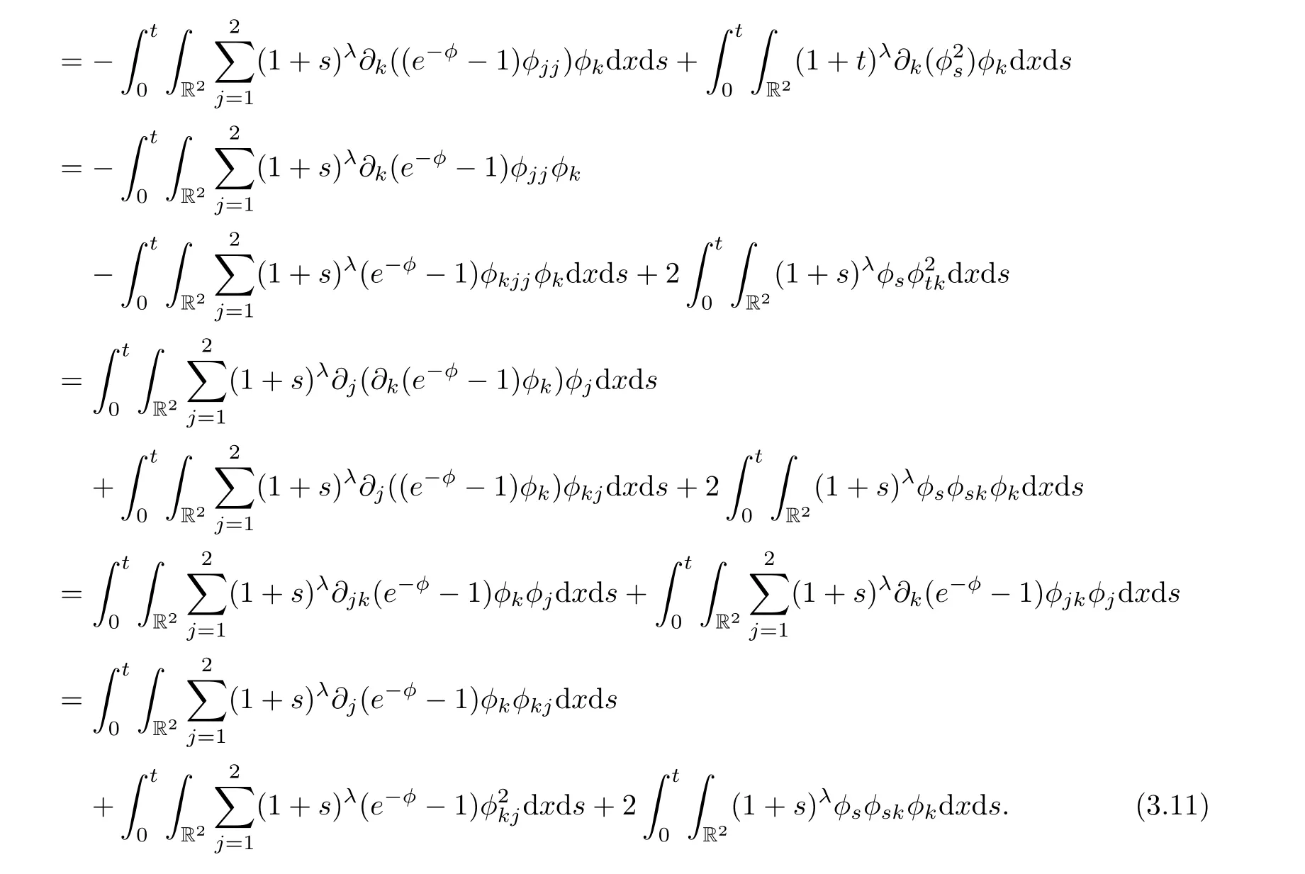
For I13,we have

thus,by(3.6),(3.8),and(3.9),we obtain

Now,we consider I2.

Thus,

By combining the above estimates,we get

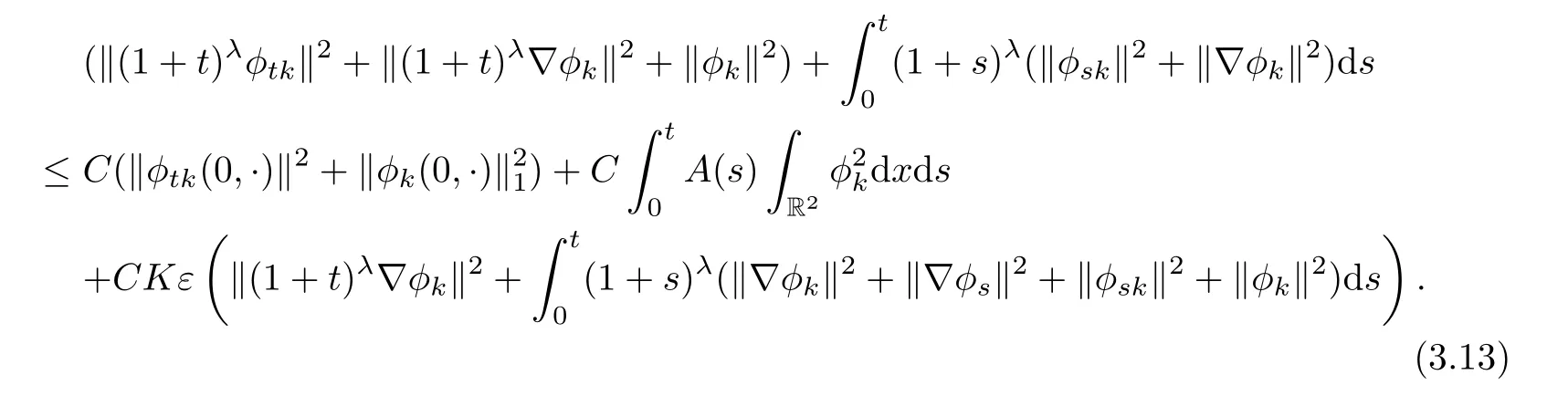
Summing k from 1 to 2,we have

provided ε small enough.

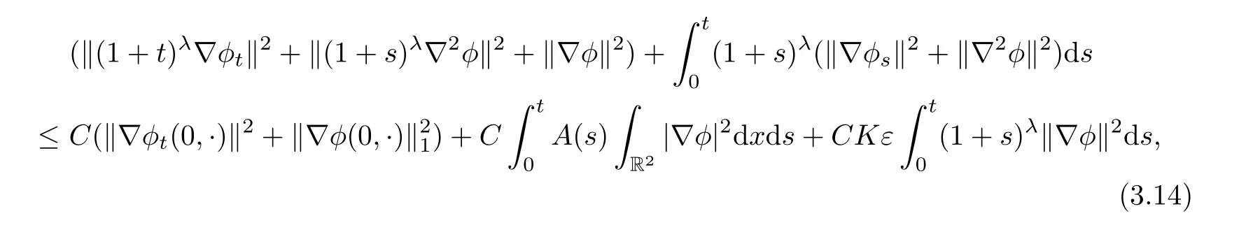
Combining(2.19)and(3.14)gives

Moreover,we can prove that for any positive number m,

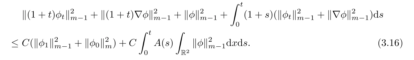
Therefore,

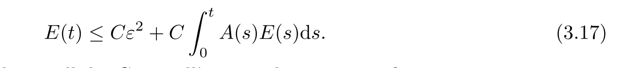
Choosing K>0 large and ε small,by Gronwall’s inequality,one get,for any t ≥ 0,

Thus,on the basis of the above discussion,we prove the main theorem 1.1 by the assumption that E(t)≤ K2ε2and a continuous induction argument.

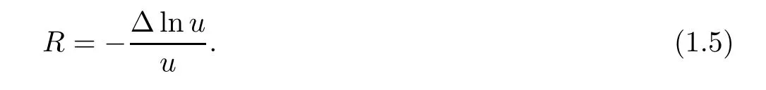
We finally estimate the scalar curvature R(t,x).By the definition,we have

Noting(1.7),we obtain from(3.19)

Using(1.14),we have

where 0< λ ≤ 1,M is a positive constant,depending on the Hsnorm of φ0(x)and the Hs−1norm of φ1(x),but independent of t and x.Thus,this prove Theorem 1.2.