EXISTENCE OF GLOBAL L∞SOLUTIONS TO A GENERALIZED n×n HYPERBOLIC SYSTEM OF LEROUX TYPE∗

Shujun LIU(刘树君)Fangqi CHEN(陈芳启),2Zejun WANG(王泽军)

1.Department of Mathematics,College of Science,Nanjing University of Aeronautics and Astronautics,Nanjing 211100,China

2.College of Mathematics and Systems Science,Shandong University of Science and Technology,Qingdao 266590,China

E-mail:numsharxy@126.com;fangqichen@nuaa.edu.cn;zjwang@fudan.edu.cn

Abstract In this article,we give the existence of global L∞bounded entropy solutions to the Cauchy problem of a generalized n×n hyperbolic system of LeRoux type.The main difficulty lies in establishing some compactness estimates of the viscosity solutions because the system has been generalized from 2×2 to n×n and more linearly degenerate characteristic fields emerged,and the emergence of singularity in the region{v1=0}is another difficulty.We obtain the existence of the global weak solutions using the compensated compactness method coupled with the construction of entropy-entropy flux and BV estimates on viscous solutions.

Key words Conservation laws;hyperbolic system;LeRoux type;viscosity method;compensated compactness

1 Introduction

In this article,we consider the Cauchy problem for two generalized(n+1)×(n+1)hyperbolic systems of LeRoux type,

and

respectively with L∞bounded measurable initial data

Systems(1.1)and(1.2)are generalized cases of the following 2×2 system of LeRoux type,

which was first studied by LeRoux in[1].

When n=2,the two characteristic fields of system(1.4)are straight lines and it is a special case of hyperbolic systems of Temple’s type,whose shock wave curves and rarefaction wave curves coincide.This system was first studied in[2],and in[3],Heibig obtained the existence and the uniqueness of L∞global solutions for general n×n hyperbolic systems of Temple type in its strictly hyperbolic region.All the results above were based on the BV boundness of the initial data.Because for systems of Temple type,this boundness can be preserved as time increasing.If we only consider the L∞initial data,the case will be more difficult because some technically constructed entropy-entropy flux are needed to apply compensated compactness method to get the pointwise convergence of approximated solutions,and this work was indeed completed by Lu et al in[4].However,if we consider the generalized n×n system(1.1)or(1.2),the emergence of more linearly degenerate characteristic fields brings us more difficulties in constructing entropy-entropy flux and passing weak convergence to pointwise convergence of approximated viscous solutions.Another obstacle is that the singularity on{v1=0}will be emerge on the right hand of the approximating viscosity systems(2.33),when we try to obtain some useful compactness estimates.So,we need new compact conditions and analysis of viscous solutions to overcome these difficulties.

2 Existence of Global Solutions to System(1.1),(1.3)

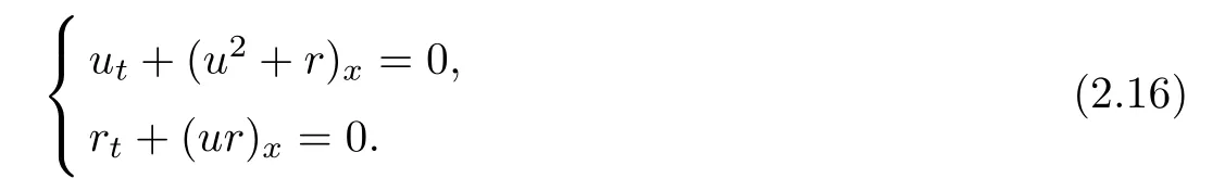
We rewrite system(1.1)as the following form,

where U=(u,v1,···,vn)Tand the coefficients Matrix has a claw type,

By a simple calculation,the n+1 eigenvalues of Matrix A(U)are

and the corresponding left and right eigenvectors are,respectively,

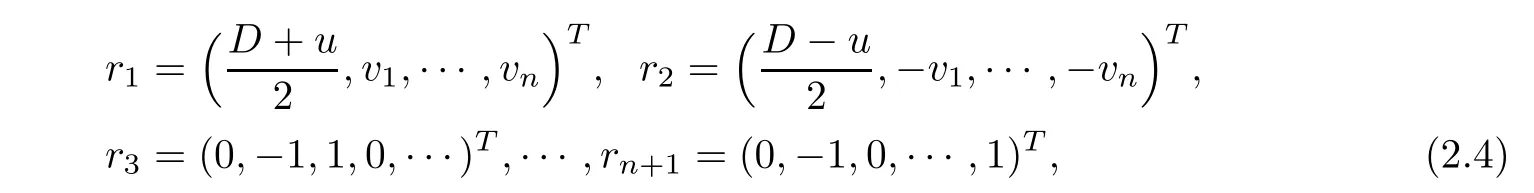
It is easy to obtain the followings,

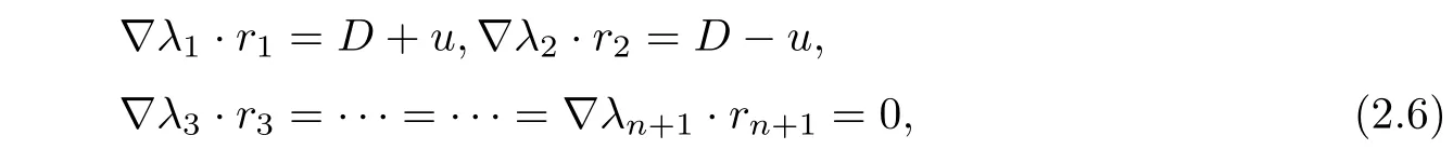
therefore system(1.1)is non-strictly hyperbolic.The first and second characteristic fields are linearly degenerate in the region{v=0,u≤0}and{v=0,u≥0},respectively,and the n−1 other characteristic fields are linearly degenerate.

Along the n−1 linearly degenerate fields,the initial oscillations can propagate as time increasing,whose property is similar to the propagation and cancelation of oscillations in the linearly degenerate field for the symmetric system of Key fitz-Kranzer[6]type first considered in[5]by Chen.For further studies,please see[12,13].So,we consider the following bounded,compactness conditions on initial data as in[7].

In this section,we avoid the construction of entropy-entropy flux of Lax’s type for system(1.1)in[4],but use a new technique to estimate the BV bounds on viscous solutions,the skills dealing with singularity given in[7],and the framework of compensated compactness principle to give the proof of the existence of L∞bounded global entropy weak solutions.

Adding viscosity terms to the right hand of(1.1),then we consider the following parabolic system

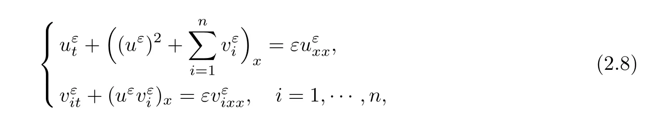
with bounded initial data

where M is a constant independent of ε.and we have the following main result,

Theorem 2.1Suppose that the initial data w1(x,0)or w2(x,0)is L∞∩ BV bounded measurable,where wi(x,t)(i=1,2)are the strict Riemann invariant as in(2.5).Condition(2.7)is satisfied.Then,Cauchy problem(2.8)–(2.9)has a global L∞bounded viscosity solutionfor any ε>0,that is,and M is a constant independent of ε.

Moreover,there exists a subsequence ofalso labeled asconverging point wisely to function(u(x,t),v1(x,t),···,vn(x,t))which is a weak entropy solution of Cauchy problem(1.1),(1.3)in the sense of Lax and we have the following estimates

Remark 1An L∞bounded vector function(u(x,t),v1(x,t),···,vn(x,t))is called a weak entropy solution of Cauchy problem(1.1),(1.3)if for any test functionthe following equalities hold:

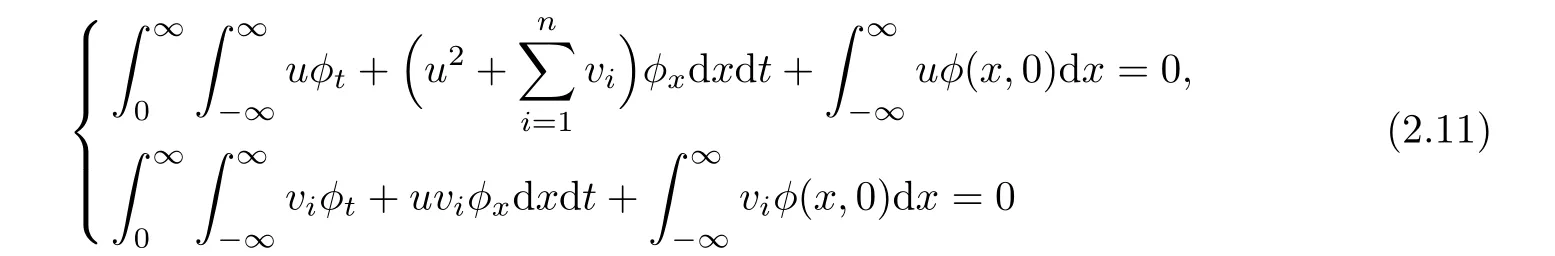
and the entropy inequality

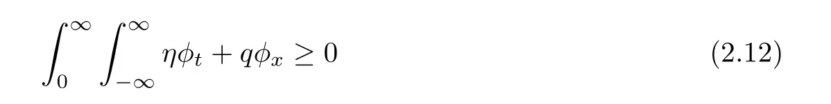
holds for any non-negative test functionswhere(η,q)=(η(u,v1,···,vn),q(u,v1,···,vn))is a pair of convex entropy-entropy flux of system(1.1),that is,the Hessian Matrix∇2η is non-negative.

Remark 2In the special case,where system(1.1)is a 2×2 system,if we take vi(x,t)≡0 for i=2,···,n,then condition(2.7)is naturally satisfied.

Next,we prove Theorem 2.1 by the following three lemmas.

Lemma 2.2If the conditions in Theorem 2.1 are satisfied,then there exist global L∞bounded viscosity solutionsfor Cauchy problem(2.8),(2.9).

ProofFirst,it is easy to obtainfor i=1,···,n,from Theorem 1.0.2(4)in[8],where c(ε,t)may tends to zero as t → ∞ or ε → 0. We denoteIf multiplying the both sides of system(2.8)withandrespectively,we have the followings,

and

Now,we avoid the technical construction of entropy-entropy flux in[4],and give the following lemma on the pointwise convergence of(uε(x,t),rε(x,t))directly by using the BV bounds of initial data.

Lemma 2.3If the conditions in Theorem 2.1 are satisfied,then there exists a subsequence of{(uε(x,t),rε(x,t))}(also labeled as{(uε(x,t),rε(x,t))})converging pointwisely to a pair of functions(u(x,t),r(x,t))which satisfies

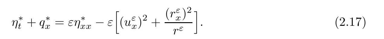
Multiplying(2.17)by a test functionwhich satisfies φ|K=1,0≤ φ ≤1 for any arbitrary compact set K⊂suppφ⊂R×R+,we get

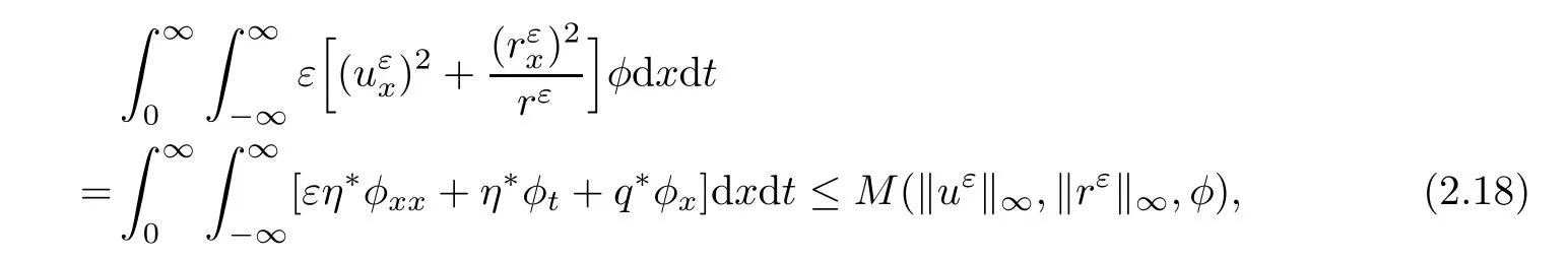
where the two terms on the left side of(2.18)both are nonnegative and then both areR+)bounded.

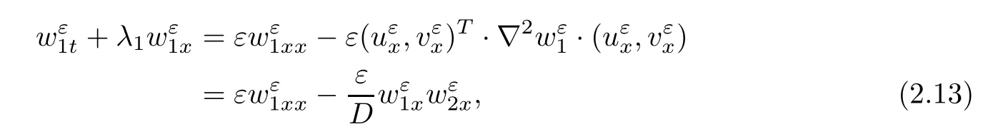
Differentiating(2.13)with respect to x and multiplying the both sides by g′(θ,α),we obtain

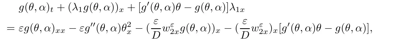
in the sense of distributions if let α→0.Integrating(2.19)in R×[0,t],we obtain

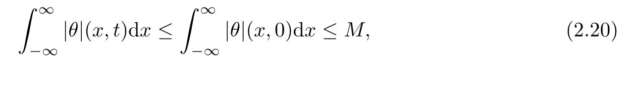
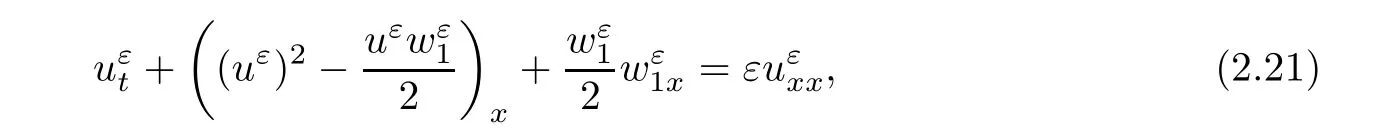
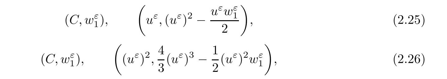
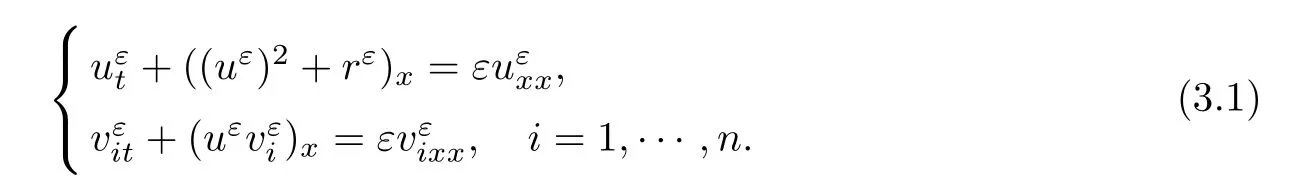
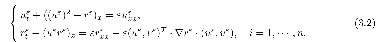
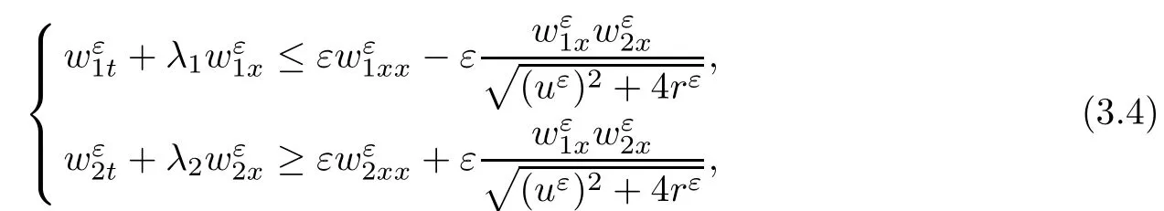
where the first and second terms on the left side of(2.21)arebounded,the third term is L1(R×R+)bounded and then(1

Multiplying(2.21)by 2uε,we have

By the same analysis,we also get

Next,we apply Div-Curl Lemma to the following two pairs of functions,respectively,

then we obtain

and obtain

for the same of(2.27),which means

As for the pointwise convergence of rε,if we apply Div-Curl Lemma to the following two pairs of functions

we obtain

for the sake of the pointwise convergence of uε,which means that rε→ r pointwisely and we complete the proof. ?

Now,we have proved the pointwise convergence of(uε(x,t),rε(x,t));and to get the pointwise convergence for eachn,we need the following lemma.

Lemma 2.4If the conditions in Theorem 2.1 are satisfied,then there exists a subsequence ofconverges to a function h(x,t)∈L∞(R×R+)pointwisely on the region{v1>0},for i=2,···,n.Moreover,the viscosity solutionshas the estimates(2.10)given in Theorem 2.1.

ProofMultiplying the second and i+1th equation of(2.8)byandrespectively,and adding the results,we have

in the sense of distributions if let α→0.Integrating(2.34)in R×[0,t],we obtain

we obtain

which indicates

Combining Lemma 2.3 and Lemma 2.4,we obtain the pointwise convergence ofon the region{v1>0}.For the region{v1=0},it holds that vi=0,i=2,···,n,from the estimates(2.10),and the global existence results is trivial.

Next,we will show that the weak solution(u(x,t),v1(x,t),···,vn(x,t))satisfies Lax entropy inequality.It is obvious that for any entropy-entropy flow(η,q),

then letting ε→ 0,we get(2.12).

3 Existence of Global Solutions to System(1.2),(1.3)

Adding viscosity terms to the right side of(1.2),we have

Multiplying∇rεto the last n equations of system(3.1)and adding the results,we obtain

Because∇2rεis nonnegative,then(3.3)can be rewritten as

and this coupled with classical existence of local solutions gives the existence and the L∞boundness of global viscosity solution(uε(x,t),rε(x,t))via the Invariant Region Principle in[9].

By the same technique of(2.17),(2.18),we can know that both

Now,we introduce four pairs of entropy-entropy flux as in[4](for simplicity we omit the subscript ε here),

and summarizing all the analysis above,we give the following theorem.

Theorem 3.1Suppose that the initial data(u0(x),v0(x))is L∞bounded measurable and condition(2.7)is satisfied.Then,Cauchy problem(3.1),(2.9)has a global L∞bounded viscosity solutionfor any ε>0,that is,≤ M,and M is a constant independent of ε.

Moreover,there exists a subsequence of(also labeled asconverging pointwisely to function(u(x,t),v1(x,t),···,vn(x,t)),which is a weak entropy solution of Cauchy problem(1.2),(1.3)in the sense of Lax,and we have the following estimates