INITIAL BOUNDARY VALUE PROBLEM FOR A NONCONSERVATIVE SYSTEM IN ELASTODYNAMICS∗
2018-07-23DivyaJOSEPHDINESH
K.Divya JOSEPH P.A.DINESH
Department of Mathematics,M.S.Ramaiah Institute of Technology MSRIT P.O,Bangalore 560054,India
E-mail:divyakj@msrit.edu;dineshdpa@msrit.edu
Abstract This article is concerned with the initial boundary value problem for a nonconservative system of hyperbolic equation appearing in elastodynamics in the space time domain x>0,t>0.The number of boundary conditions,to be prescribed at the boundary x=0,depends on the number of characteristics entering the domain.Because our system is nonlinear,the characteristic speeds depends on the unknown and the direction of the characteristics curves are known apriori.As it is well known,the boundary condition has to be understood in a generalised way.One of the standard way is using vanishing viscosity method.We use this method to construct solution for a particular class of initial and boundary data,namely the initial and boundary datas that lie on the level sets of one of the Riemann invariants.
Key words Elastodynamics;viscous shocks
1 Introduction
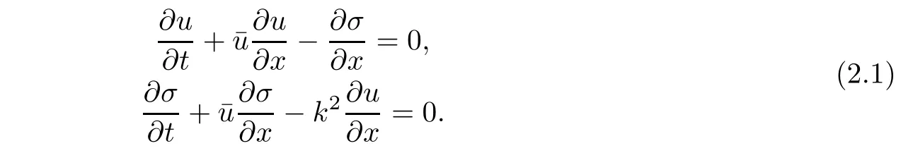
In this article,we study a system of two equations,appearing in elastodynamics,namely,
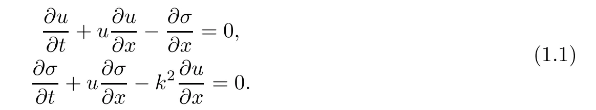
Here,u is the velocity,σ is the stress,and k>0 is the speed of propagation of the elastic waves and the system corresponds to the coupling of a dynamical law and a Hooke’s law in a homogeneous medium in which density varies slightly in the neighborhood of a constant value.In fact,this system was derived in[2]as a simplification of a system of four equations of elasticity describing mass conservation,momentum conservation,energy conservation,and Hooke’s law.
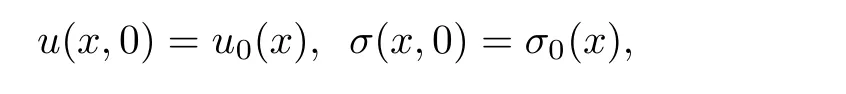
Initial value problem for system(1.1)is well studied by many authors[2,3,6,7],however,the boundary value problem is not understood well.The aim of this article is to study initial boundary value problem for(1.1),in x>0,t>0 with initial conditions

and a weak form of the boundary conditions,

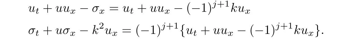
We write(1.1)as the system
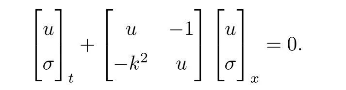
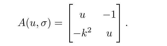
Let us denote
System(1.1)is non-conservative because it cannot be written in the conservative form,namely,
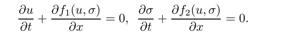
In other words,there does not exist f:R2→R2such that
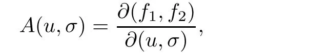
where f(u,σ)=(f1(u,σ),f2(u,σ)).The eigenvalues of A(u,σ)are called the characteristic speeds of system(1.1).A simple computation shows that the equation for the eigenvalues are given by
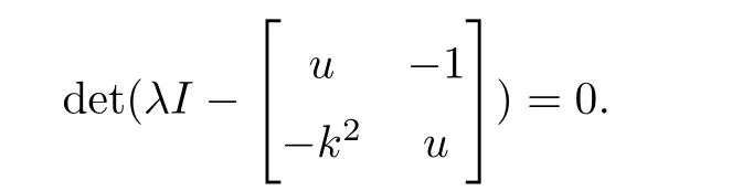
This gives

which has two real distinct roots and so the system is strictly hyperbolic.We call λ1the smaller one and λ2larger one,then we have


We say wi:R2→R is a i-Riemann invariant if
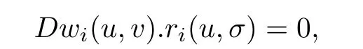
where Dwi(u,v)=(wiu,wiσ)is the the gradient of wiw.r.t.(u,σ)and ri(u,σ)is a right eigen vector corresponding to the i-th characteristic speed λi(u,σ).First,we prove a few basic properties of Riemann invariants.For the special system that we are studying,these two families of Riemann invariants can be constructed globally and they play an important role in our analysis.

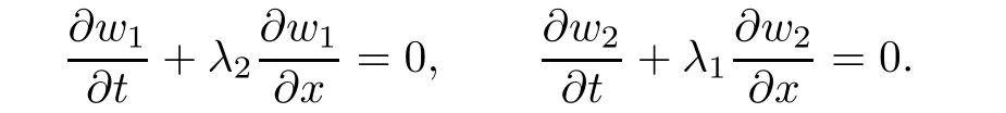
LemmaThe functions w1and w2given by are 1-Riemann invariant and 2-Riemann invariant respectively.Furthermore,w1is constant along 2-characteristic curve and w2is constant along 1-characteristic curve.
ProofBy the definition,w1(u,σ)is a 1-Riemann invariant if w1u+kw1σ=0 and w2(u,σ)2-Riemann invariant if w2u−kw2σ=0.Now,w1u+kw1σ=0 gives w1(u,σ)= φ1(σ−ku),where φ1:R1→ R1is arbitrary smooth function,whereas w2u−kw2σ=0 gives w2(u,σ)= φ2(σ+ku),φ2:R1→ R1.In particular,taking φ(w)=w,we get the pair of Riemann invariants as given in Lemma.An easy computation shows that

This,together with(1.1),after rearranging the terms,gives
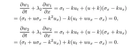
In short,
Let xi=βi(t)be an i-characteristic curve.We have
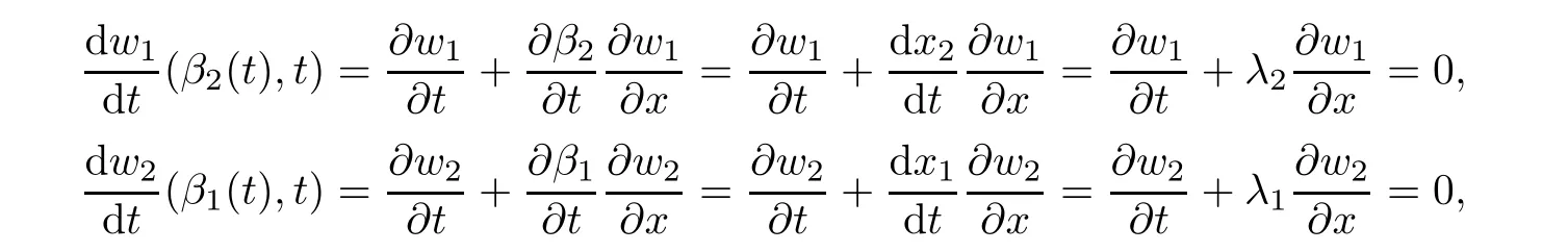
which proves the lemma.
2 Initial Boundary Value Problem for the Linearized System
In this section,we study initial boundary value problem for the linearized system of(1.1)around a constant state.Let

Writing this in Riemann invariants,we get

whose general solution is

for any functions φi:R → R,i=1,2.
Now,we consider the initial boundary value problem in x>0,t>0,with initial condition
and boundary condition
In Riemann invariant,they take the form

and

respectively.The boundary conditions at x=0 can be prescribed only if both+k and−k are positive.
To understand the situation,consider the equation

where λ is constant.The general solution to this PDE is a= φ(x − λt),which is the unique solution of this PDE with initial condition a(x,0)=φ(x).Now,if we look at the initial boundary value problem in the quarter plane x>0,t>0,with initial data at t=0,the solution is uniquely determined if λ<0 because any characteristic curve through(x,t),x>0,t>0 can be drawn back to the initial line,that is,the x-axis at a point y=x−λt and a(x,t)=a(x−λt,0).So,no boundary conditions are required at x=0.On the other hand,if λ>0,then all the characteristic lines at x=0 are pointing inwards the domain x>0,t>0,and then the initial data,a(x,0)=a0(x),x>0,determine the solution in the region x>λt.The boundary condition a(0,t)=ab(t)is required to determine the solution in 0
Case 1λ<0
Here,no boundary condition is required.The characteristic curve is x=λt+y,a(x,t)=a0(x−λt);
Case 2λ>0
In this case,the boundary condition a(0,t)=ab(t)is required.The characteristic curve is x=λt+y.
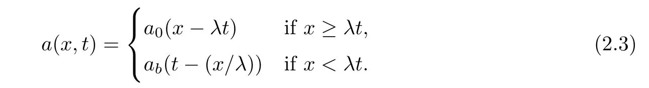
If x ≥ λt,we have a(x,t)=a0(x − λt).If x< λt,a(x,t)=a(0,τ),where(0,τ)is the point of intersection of the characteristic passing through(x,t)with slope λ and the t-axis.So a(x,t)=ab(τ)=ab(t− (x/λ)).So the solution is
Now,getting back to system(2.1),or equivalently(2.2),the following cases occur.
Case 1
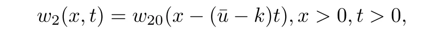
In this case,the initial data w1(x,0)=w10(x),w2(x,0)=w20(x)determine the solution and no conditions are required on x=0 and explicit solution in x>0,t>0 is given by

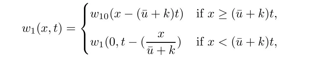
Case 2and
Here,apart from the initial conditions as above,one condition is required.This is of the form
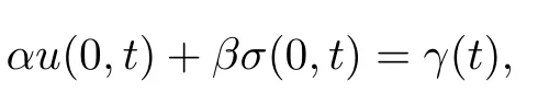
where γ(t)is a given function of t and α,β are constants withIn Riemann invariants,this is equivalent to
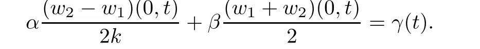
So,we have

and from(2.3),

which implies

Rewriting,we get

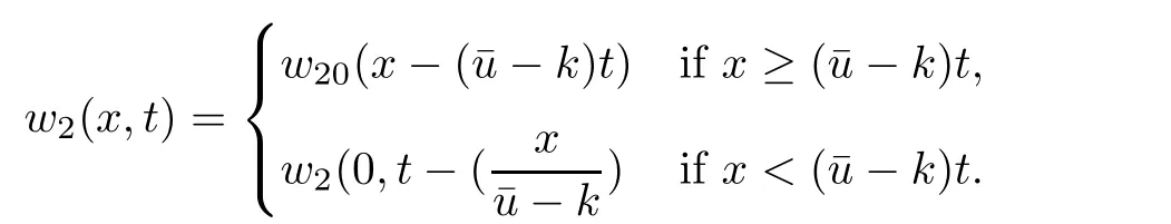
Case 3


and

From(2.3),we have
and
Note that(2.5)and(2.6)can be written as
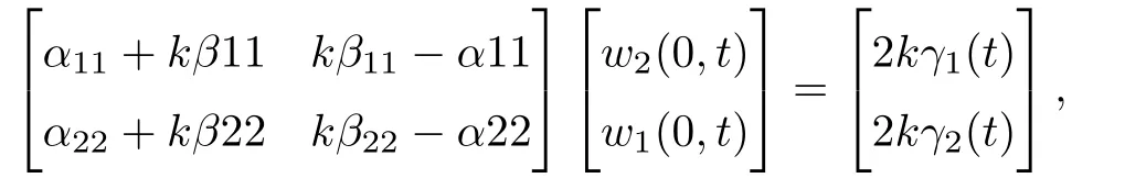
which can be solved if
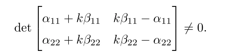
An easy computation shows that this is equivalent to

By simplification,
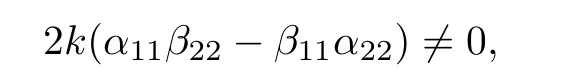
that is,

which we have assumed earlier.A special case is α11=1,β11=0 α22=0,β11=1,which is the Dirichlet’s Boundary condition u(0,t)= γ1(t),σ(0,t)= γ2(t).
3 Initial Boundary Value Problem When the Data is on the Level Set of Riemann Invariants
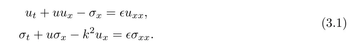
System(1.1)is nonconservative and strictly hyperbolic with characteristic speeds λ1(u,σ)=u−k,λ2(u,σ)=u+k and it is well known that smooth global in time solutions does not exist even if the initial data is smooth.As the system is nonconservative,any discussion of wellposedness of solution should be based on a given nonconservative product in addition to the admissibility criterion for shock discontinuities.Indeed,the system is an approximation and is obtained when one ignores higher order terms,which give smoothing effects with small parameters as coefficients.So,the physical solution is constructed as the limit of a given regularization as these parameters goes to zero.Different regularizations correspond to different nonconservative product and admissibility condition.In this article,we take a parabolic regularization,
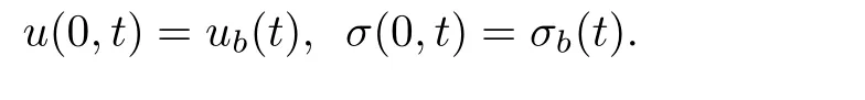
This approximation is particularly useful in the study of the initial boundary value problem for(1.1)in x>0,t>0,as we cannot prescribe initial and boundary conditions,

for(1.1)in the strong sense.
In this section,we consider the initial boundary value problem for(1.1)with initial condition(1.2)and a weak form of the boundary condition(1.3)when initial and boundary data lie on the level set of one of the Riemann invariants.We take the data to be on the level set of the j-Riemann invariant and therefore

where c is a given constant.Throughout this section,we assume that u0,σ0are bounded measurable and ub,σbare continuous.We look for a solution of the form σ = −(−1)jku+c;substituting this in(1.1),we get

This gives
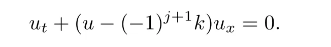
Making the substitution v=u−(−1)j+1k,problem(1.1)is reduced to

The boundary condition v(0,t)=ub(t)−k cannot be satisfied in general;in the strong sense that as the characteristics depends on the solution and at the boundary point,the characteristics may point out of the boundary when drawn in increasing time direction.We construct the solution u(x,t)as the limit of uǫ(x,t)as ǫ→ 0 for(3.1)with initial and boundary conditions(3.2)
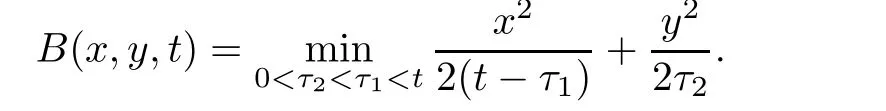
To describe the vanishing viscosity limit,we need to introduce some notations.First,we introduce a functional defined on a certain class of paths;that is described in the following way.For each fixed(x,y,t),x ≥ 0,y≥ 0,t>0,C(x,y,t)denotes the following class of paths β in the quarter planeEach path is connected from the point(y,0)to(x,t)and is of the form z= β(s),where β is a piecewise linear function of the maximum three lines.On C(x,y,t),we define a functional

We call β0straight line path connecting(y,0)and(x,t)which does not touch the boundary x=0,namely,{(0,t),t>0},then let

Any β ∈ C∗(x,y,t)=C(x,y,t)− {β0}is made up of three pieces of lines connecting(y,0)to(0,τ1)in the interior,(0,τ1)to(0,τ2)on the boundary,and(0,τ2)to(x,t)in the interior;or two pieces with one straight line in the interior and another on the boundary,and passing through(0,0).
For such curves,it can be easily seen that

In the case,where τ1=0,y=0,

It was proved in[8]that there exists β∗∈ C∗(x,y,t)and corresponding τ1(x,y,t),τ2(x,y,t)such that
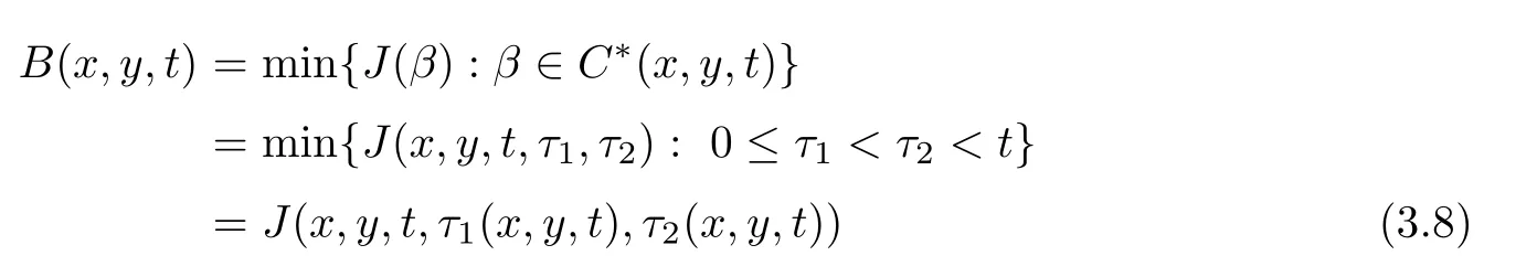
is Lipshitz continuous.Furthermore,it was also proved that

and

are Lipshitz continuous function in their variables,where

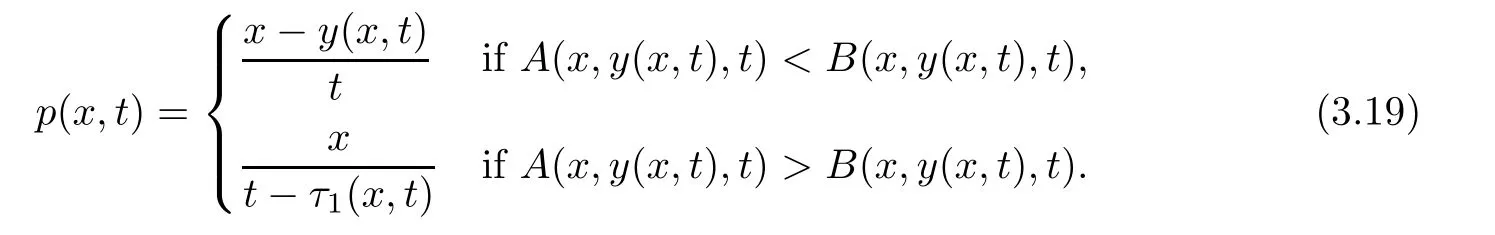
Furthermore,the minimum in(3.10)is attained at some value of y≥0,which depends on(x,t);we call it y(x,t).If A(x,y(x,t),t)≤B(x,y(x,t),t),

and if If A(x,y(x,t),t)>B(x,y(x,t),t),

Here and hence forth,y(x,t)is a minimizer in(3.10)and in the case of(3.12),τ2(x,t)=τ2(x,y(x,t),t)and τ1(x,t)= τ1(x,y(x,t),t).With these notations,we have an explicit formula for the solutions of(1.1)and(1.2)with a weak form of the boundary condition(1.3),as the vanishing viscocity limit of(3.3)–(3.4)is given by the following result.
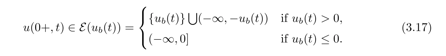
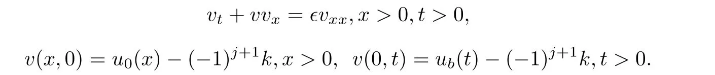
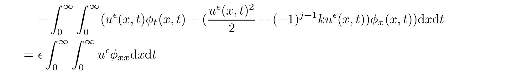
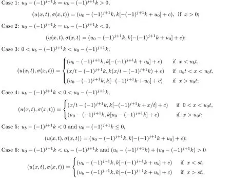
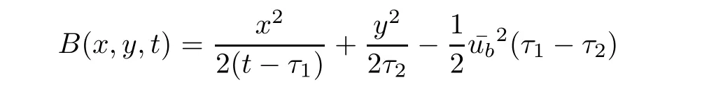
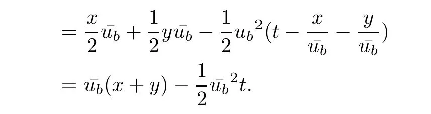
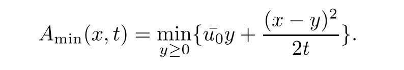
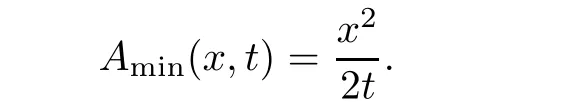
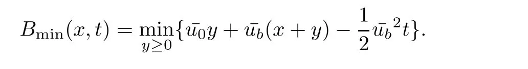
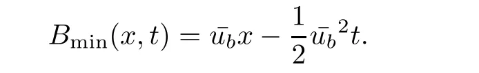
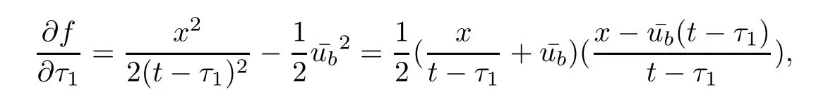
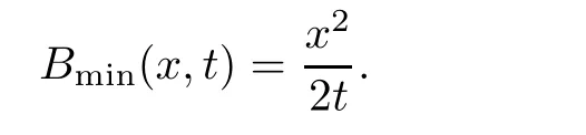
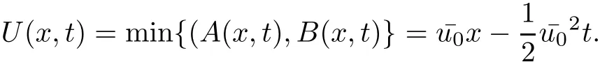
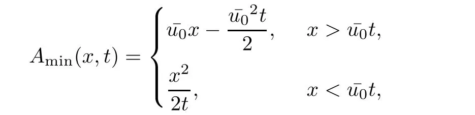
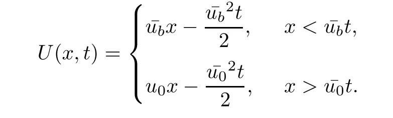
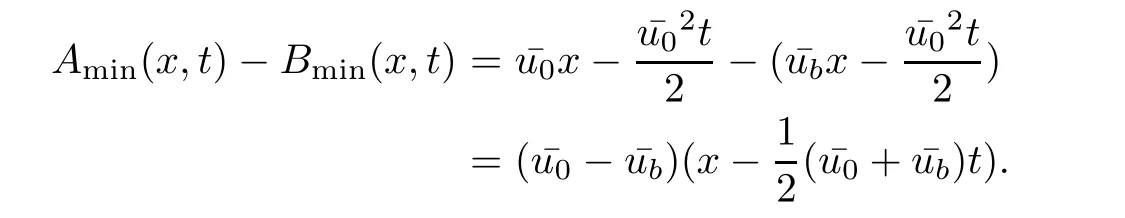
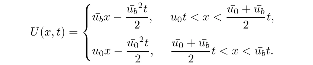
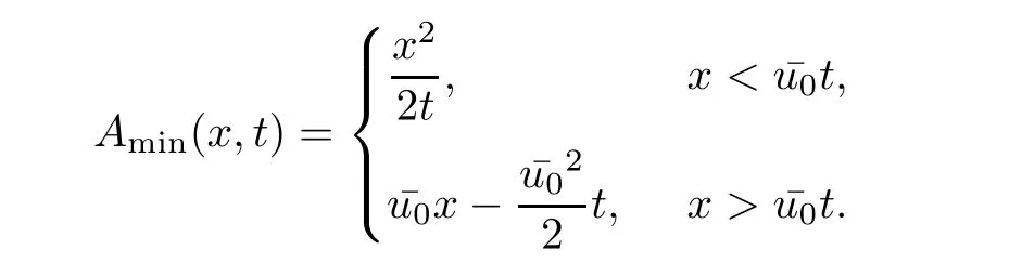
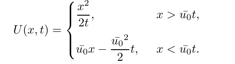
Theorem 3.1For every(x,t),x>0,t>0,the minimum in(3.10)is achieved by some y(x,t)(may not be unique)and U(x,t)is a Lipschitz continuous.Furthermore,the limitexists and has the following representation.For almost every(x,t),there exists a unique minimum y(x,t)and either A(x,y(x,t),t) Then, Furthermore(u(x,t),σ(x,t))is a weak solution of of(1.1),with initial conditions(1.2). ProofWe try to find a solution which lies on the level set of the Riemann invariant satisfying the initial and boundary conditions.When σ =(−1)j+1ku+c,system(3.3)become a single Burgers equation with initial conditions and boundary conditions A more general type of initial boundary value problem of this type was studied by Bardos,LeRoux,and Nedelec[1]and they proved the convergence of the limit as ǫ goes to 0.They further showed that the limit satisfies the equation the initial condition(3.15),and a weak form of the boundary condition(3.16),namely, Here,our aim is to get the formula for the limit.So,taking v=u−(−1)j+1k,the equation can be written as Applying Hopf-Cole transformation[4], the problem is reduced to with initial conditions and boundary conditions Existence of solution w(x,t)for this problem is well known and from the transformations,we get The formula then follows from(3.18)and(3.19). For the completeness of the arguement,we show that the limit satisfies equation(1.1).For this, first we note that the system is equivalent to in weak sense,when(u,σ)lies on one of the Riemann invariant.This follows easily because,if σ(x,t)=(−1)j+1ku(x,t)+c, Now,as uǫis smooth,it satisfies for any smooth function with compact support in x>0,t>0. As u0is bounded measurable and ubis continuous,by the maximum principle,uǫis bounded in[0,∞)× [0,T]and pointwise convergent almost everywhere.So by passing to the limit as ǫ tends to zero and using the Dominated convergence theorem,we obtain Thus,this completes the proof. RemarkThe limit in the theorem satisfies the initial conditions, but the boundary conditions at x=0, is not satified in the strong sense.Indeed,with strong form of Dirichlet boundary conditions,there is neither existence nor uniqueness,because the speed of propagation λj(u,σ)=u+(−1)jk does not has a definite sign at the boundary x=0.We note that the speed is completely determined by the first equation.However,the boundary conditions are satisfied in the sense of Bardos Leroux and Nedelec[1],which for our case is equivalent to the following condition,seeing LeFloch[9], Also,the solution satisfies the entropy condition u(x−,t)≥ u(x+,t),which follows from the formula derived in Theorem 3.1. In this section,we find an explicit formula for global solution of(1.1)when the initial data(1.2)and the boundary data(1.3)are of Riemann type. We have the following formula for the vanishing viscosity limit. Theorem 4.1Let uǫand σǫbe given by(3.18),with u0,σ0,ub,σball being constants and lying on the level sets of the j Riemann invariants,thenexists pointwise a.e.andin the sense of distributions and(u,σ)have the following form: ProofFor simplicity,denoteFix(x,y,t),x≥0,y≥0,t≥0.For 0≤τ2≤τ1 We find the minimum with respect to τ1and τ2.Note that as τ1goes to t or τ2goes to 0,f goes to infinity if x>0 and y>0,respectively.So,for this case,the minimum is inside 0< τ2≤ τ1 Now,consider Denote by g(y)the function inside the bracket,thenin the region Let Because the function inside the bracket is an increasing function of y,the minimum is achieved for y=0,so that which is positive.So,as a function of τ1,f is an increasing function and so its minimum is achived at τ1=0.This means that Bmin(x,t)is achived at τ1= τ2=y=0,such that As in previous case, so that In the region x>u0t,as before, From the first derivative condition,it is easy to see that the minimum in Amin(x,t)is achieved for y=x−0t and so and Same analysis as before gives The right-hand side is positive ifand negative ifand we get Thus,this completes the proof.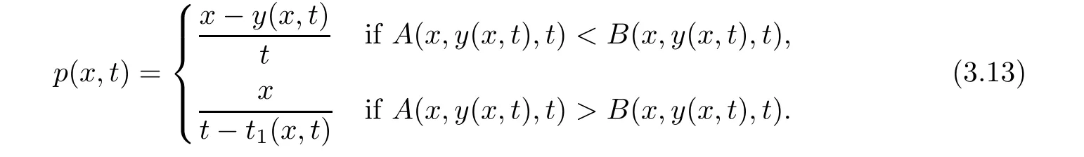


4 Initial Boundary Value Problem With Riemann Type Boundary Conditions


杂志排行

Acta Mathematica Scientia(English Series)的其它文章
- GLOBAL EXISTENCE OF CLASSICAL SOLUTIONS TO THE HYPERBOLIC GEOMETRY FLOW WITH TIME-DEPENDENT DISSIPATION∗
- NONNEGATIVITY OF SOLUTIONS OF NONLINEAR FRACTIONAL DIFFERENTIAL-ALGEBRAIC EQUATIONS∗
- GROWTH AND DISTORTION THEOREMS FOR ALMOST STARLIKE MAPPINGS OFCOMPLEX ORDER λ∗
- EXACT SOLUTIONS FOR THE CAUCHY PROBLEM TO THE 3D SPHERICALLY SYMMETRIC INCOMPRESSIBLE NAVIER-STOKES EQUATIONS∗
- PRODUCTS OF RESOLVENTS AND MULTIVALUED HYBRID MAPPINGS IN CAT(0)SPACES∗
- CONVERGENCE FROM AN ELECTROMAGNETIC FLUID SYSTEM TO THE FULL COMPRESSIBLE MHD EQUATIONS∗