Quantitative Electrophilicity Measures

GONZÁLEZ Marco Martínez, CÁRDENAS Carlos, RODRÍGUEZ Juan I., LIU Shubin,HEIDAR-ZADEH Farnaz, MIRANDA-QUINTANA Ramón Alain, AYERS Paul W.

1 Laboratory of Computational and Theoretical Chemistry, Faculty of Chemistry, University of Havana, Havana 10400, Cuba.

2 Departamento de Química, and Centro de Química Universidade de Coimbra, 3004-535 Coimbra, Portugal.

3 Departamento de Física, Facultad de Ciencias, Universidad de Chile, Casilla, 653 Santiago, Chile.

4 Centro para el desarrollo de la Nanociencias y Nanotecnología, CEDENNA, Av. Ecuador 3493, Santiago, Chile.

5 Escuela Superior de Física y Matemáticas, Instituto Politécnico Nacional, Edificio 9, U.P. A.L.M., Col. San Pedro Zacatenco,C.P. 07738, Ciudad de México, México.

6 Research Computing Center, University of North Carolina, Chapel Hill, NC 27599-3420, USA.

7 Department of Chemistry & Chemical Biology; McMaster University; Hamilton, Ontario L8S 4M1, Canada.

8 Department of Inorganic and Physical Chemistry, Ghent University, Krijgslaan 281 (S3), 9000 Gent, Belgium.

9 Center for Molecular Modeling, Ghent University, Technologiepark 903, 9052 Zwijnaarde, Belgium.

1 Introduction

The concepts of electrophilicity and nucleophilicity are cornerstones of our understanding of chemical reactivity1,2.Usually, they are merely considered in a qualitative way,together with the notions of electron accepting/donating groups, to rationalize chemical reactivity trends. However, their remarkable utility has also inspired researchers to find ways to quantify the electrophilic and nucleophilic character of a given molecule. These efforts have deepened our understanding of what makes a compound a better or worse electrophile/nucleophile, how these properties could be tuned,and how they relate to other quantities. We view the work of Mayr et al.3–7as especially important. These authors have established electrophilicity and nucleophilicity scales by means of extensive experimental tests. The defining element of these studies is the following expression:

where k20 °C is the rate constant of the reaction (at 20 °C)between the nucleophile and the electrophile, while s and N Mayr are parameters specific to the former, and E Mayr to the latter.Analyzing several combinations of electrophile-nucleophile pairs, the corresponding parameters can be determined. These definitions of the nucleophilicity and electrophilicity is clearly based on the concept that strong electrophiles react with strong nucleophiles rapidly and vigorously, while weak electrophiles and weak nucleophiles react slowly and reluctantly, if at all.

Parallel to these experimental determinations, there is steadfast interest in finding mathematical equations to quantify the electrophilicity of a molecule8–10. Perhaps the best example of this is the early work of Maynard et al.11, which proposed a simple expression for the electrophilicity in terms of electron attachment/removal energies. Parr et al.12then provided a theoretical justification for Maynard’s proposal within the framework of conceptual density functional theory (c-DFT)13–23.This landmark contribution gave chemists a simple, yet powerful, tool that has been successfully applied to the analysis of regioselectivity of cycloaddition reactions24–27, the study of leaving groups28,29, transition states30–32, and redox reactions33–35.This c-DFT electrophilicity measure has also been used as a descriptor in several quantitative structure activity relationship(QSAR) studies36–39. But arguably the biggest impact of the precise quantitative definition of the electrophilicity is that it provided a way to prove the minimum electrophilicity principle(MEP)40–44. Expanding on Parr’s work, and also within the c-DFT formalism, Gázquez et al.45, and Chamorro et al.46,47have generalized this index. Recently, new working expressions for this index has been proposed, which are free from some inconsistencies found in previous versions48,49.

The proliferation of theoretical electrophilicity measures makes it desirable to assess their performance. This is main goal of this work. As a reference for comparison, we will use Mayr’s parameter. Since the theoretical and experimental measures of electrophilicity refer to different effects, we do not expect them to be exactly the same. However, we believe that a good theoretical measure of electrophilicity must capture the trends from Mayr’s work. In addition to testing existing theoretical definitions, we will also attempt to use machine learning techniques to find a mathematical expression that reproduces the Mayr electrophilicity.

2 Conceptual DFT electrophilicity measures

Parr et al.12defined the electrophilicity, ω, as the stabilization energy associated with the electronic saturation of the system (e.g., molecule). In other words, how the energy of a system changes when it reaches equilibrium with a perfect electron donor. Evaluating this definition requires a model for how the electronic energy, E, changes with respect to the number of electrons, N. If we neglect the changes in the external potential (e.g., molecular geometry) during the electron saturation process, we can estimate energy variation in terms of the following (truncated) Taylor expansion50:

Within the c-DFT framework is customary to identify the coefficients of this expansion with different reactivity descriptors. For example, Parr et al.51proposed to identify the coefficient of the linear term with the (electronic) chemical potential of the system, μ, which is in turn defined as the additive inverse of the electronegativity, χ:

In a similar way, Parr and Pearson50identified the coefficient of the quadratic term with the chemical hardness, η,which is in turn defined as the multiplicative inverse of the chemical softness, S:

In c-DFT, a perfect electron donor is defined as a system with zero electronegativity (e.g., zero chemical potential). This means that Parr’s electrophilicity definition can be written as:

where μ0is the chemical potential of the isolated system.

The standard way to approximate this index is to notice that,according to Sanderson’s electronegativity equalization principle52, the system will reach electronic saturation when:

Substituting Eq. (2) in this expression we can calculate the maximum number of bound electrons, ΔNmax:

From this it is now easy to see that:

Notice that we have explicitly indicated that this expression corresponds to the quadratic energy model used in Eq. (2). (It is possible to generalize this expression to differentiate between the electrophilicity of spin up and spin down electrons53–60, but this will not be considered here.)

To obtain a working expression for the electrophilicity we need to express the chemical potential and chemical hardness in terms of quantities from electronic structure theory that can be computed using standard quantum chemistry software. This can be done by viewing Eq. (2) as a parabolic interpolation of the electronic energy of the system with N0, N0+ 1, and N0− 1 electrons or, equivalently, using a three-point finite differences approximation with ΔN = 161:

here, I and A are the ionization energy and electron affinity,respectively. Substituting these expressions in Eq. (8) we obtain:

Motivated by the success of the parabolic model, Gázquez,Cedillo, and Vela (GCV) proposed a two-parabolas model that allowed them to describe electron transfer processes in a more realistic way45. The key insight in their work was to distinguish between the electron-accepting and the electron-donating processes. (Since we will be only concerned here with the ability of a system to incorporate electron, we will neglect the latter.) In their formulation, the electron-rich and electron-poor regimes are described by different parabolas(e.g., different E vs N models) with the same curvature.Imposing different conditions on this simple model, they obtained the expressions for the chemical potentials of the system when is gaining, μ+GCVelectrons:

Their model is completed with the assumption that the chemical hardness for both electron-accepting and electron-donating processes is equal:

These new expressions can be substituted in the general working equation obtained by Parr (cf. Eq. (8)), resulting in the following electroaccepting, ω+GCV, power45:

Inspired by the work of GCV, Chamorro, Duque, and Pérez(CDP)46,47rewrote Eq. (8) using the electron accepting, μ+,chemical potential obtained from the piecewise linear interpolation of Perdew, Parr, Levy, and Balduz62:

Therefore, they obtained:

Additionally, these authors also proposed a simpler ansatz,where the chemical hardness of a system gaining electrons could be related to the chemical potential of the inverse process. In other words, making46,47:

Recently, it has been pointed out that there are several problems with the classical way to calculate the electrophilicity,Eq. (11)49. Most notably, this formula gives unreasonable results for polycations (where ΔNmax＞＞ 1) and for species with small electron affinities (where ΔN max should be close to zero,but may not be). These, and other, problems could be traced back to the fact that while the parabolic interpolation is mathematically consistent63, it lacks a rigorous physical justification64,65(except for some cases)66,67. This situation motivated the analysis of the electrophilicity index using a finite temperature formulation of the grand-canonical ensemble(an approach that has provided rigorous foundations to several c-DFT results)48,68–75. Within this formulation, it is easy to obtain an exact working expression that preserves the physical meaning of Parr’s definition. This thermodynamic electrophilicity, ωTD, is simply given by49:

From here results:

whereis the k th electron affinity of the system with M0particles, and θ(x) is Heaviside (step) function. If we are only considering the same three states used in the parabolic model(e.g., “neutral”, “cationic”, and “anionic” states), this result is reduced to:

This merely takes the electrophilicity to be equal to A when A ＞ 0, and zero in the other cases. This is the simplified expression that we will be using in the following.

Finally, it has been also shown that a consistent description of chemical reactivity within c-DFT requires the descriptors to incorporate the effects of the molecular surroundings75–79. The simplest way to do so is using the insights obtained from the Klopman-Salem frontier molecular orbital treatment80–86,which allows us to obtain model expressions for the perturbed chemical potential, μP, and the perturbed chemical hardness,ηP76:

where γ and ζ are non-negative parameters that model the interaction with the environment. Including these modified descriptors in Eq. (8) we obtain a more general, perturbed electrophilicity, ωP:

In the following, we will analyze how the previously discussed electrophilicity measures correlate with Mayr’s electrophilicity parameter. To do this, we will work with a simple linear correlation:

Since the effect of thefactor in Eq. (23) can be included in the slope, m, of the linear regression, we will work with a simplified version of the perturbed electrophilicity,namely:

3 Electrophilicity measures from symbolic regression (SR)

The indices presented in the previous section are chemically motivated and, as such, they help us determine the factors which govern the acceptance of electrons by an electrophile.While this is a valuable approach, sometimes we are more interested in obtaining an accurate estimate of the electrophilicity, regardless of the insight, it might provide. An attractive alternative in this respect is the use of machine learning (ML) tools87–91.

Here, we will work with a very powerful data mining tool:symbolic regression (SR)92–100. SR is a supervised method,which means that we provide the algorithm with a “training set” in order to find correlations between different descriptors and a property of interest. The goal of SR is to use a training set to obtain a mathematical function that relates the desired properties to the data. In this way, SR gives the best functional form (of a given pre-specified complexity), along with the best numerical parameters, for a given training set. In more technical terms, given a set of data values(training set),withrepresenting a vector of independent variables (e.g.,descriptors), and→ y the dependent variable (which will be predicted from x), SR finds the function y = fthat best describes the overall data. The optimization process takes place over a function space, expanded by mathematical operators and constants100. If the function space includes all possible functional forms, that is, the length of the mathematical expression can go up to infinity and there is no restriction on the operators used, the method will find many different functions which fit all the data exactly. However, this might cause problems when describing points/observations outside the training set. It is therefore common to enforce some constraints during the SR procedure (e.g., the length of the functions, the number of operands and numerical parameters used, etc.)

Once we restrict the accessible function space, an intuitive choice would be to select a set of basis functions to expand it.However, while this will turn the SR problem into a more familiar linear regression, the size of the basis needed makes this impractical in most cases. This demands the use of different optimization methods, with evolutionary algorithms being a popular choice. Here we will focus on two such algorithms: genetic programming (GP)100–103and grammatical evolution (GE)104–106.

3.1 Genetic programming (GP)

Genetic programming (GP)100–102draws inspiration from the mechanism of DNA replication, with new “generations” (e.g.,functional forms) leading towards better solutions. On this algorithm, each possible solution is referred to as an“individual”. In the case of an SR, these are functions proposed to fit the data. These individuals are commonly represented as a tree (see Fig. 1). The leaves represent constants or data variables, and the nodes represent the allowed mathematical operators. It is important to remark that it is possible if desired,to use basically any function as an operator, and not only the four basic arithmetic operators.

The algorithm starts with a random generation of possible solutions (trees) that fulfill the restrictions imposed (e.g., the operators allowed and the maximum length of the solution).Then, a new generation of solutions is created, following three steps: breeding, evaluation, and selection. The breeding involves the creation of a new set of alternative solutions. This can be done in several ways107: copying a solution to the new generation; combining two solutions to produce two new ones by exchanging two randomly selected subtrees between the parents (crossover)108; changing part of a solution (subtree) for a new, randomly generated, one (mutation)103(see Figs. 2 and 3). The crossover operator ensures that the individuals of the new generation share characteristics of their parents; while the mutation process prevents premature convergence of the algorithm by adding randomness. These changes occur in an uncontrolled way. Then, the evaluation step consists in the evaluation of the fitness function for each of the newly created candidate solutions. The last step consists of the selection of some of the newly created solutions in order to conform the population of the new generation. The probability to select an individual increases with the quality of the fitness calculated in the evaluation step. This process is repeated until a termination criterion is fulfilled (typically given by the number of iterations or a fitness threshold).

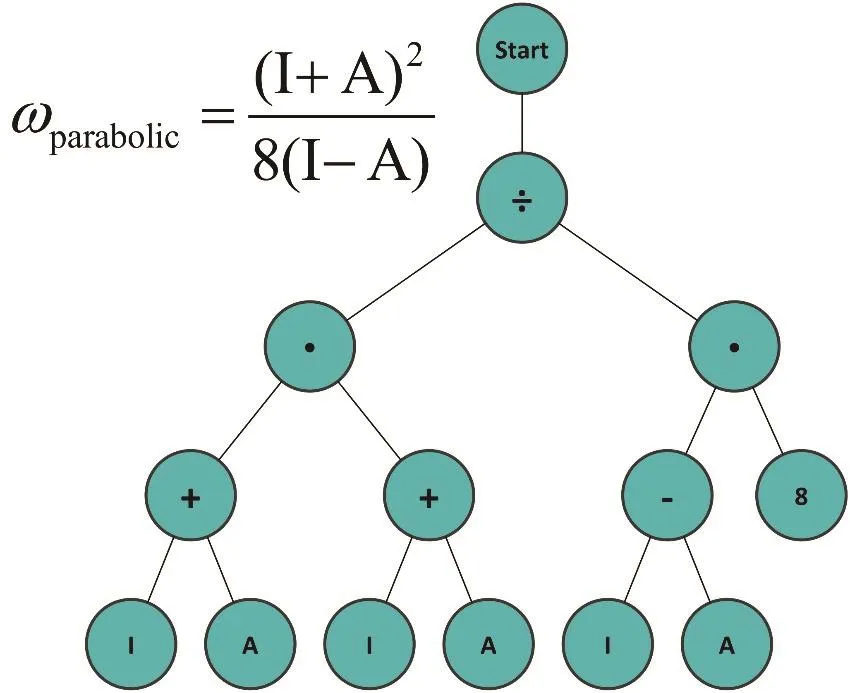
Fig. 1 Tree representation of Parr’s electrophilicity equation.

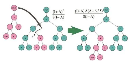
Fig. 2 Effect of the mutation operator on a tree.

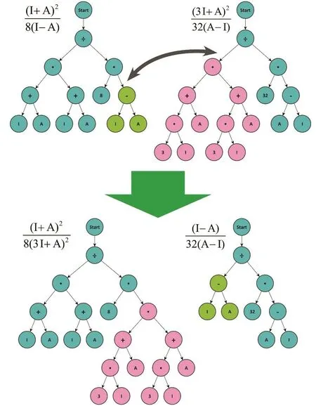
Fig. 3 Effect of the crossover operator on two trees.

3.2 Grammatical evolution (GE)

Grammatical evolution (GE)104–106, a more recent evolutionary algorithm, uses a grammar to map an integer array into a program (in the case of an SR, into a function). To do the mapping, GE uses a context-free grammar109–111, which along with an alphabet of terminal symbols, a set of non-terminal symbols, production rules, and a start symbol, is capable of deriving a model from an integer string. These integer strings are then optimized by an evolutionary technique. At every step,the composition rules are used to map from the array to the corresponding model, in order to evaluate the fitness of the latter. This resembles the natural process in which the genotype is separated from the phenotype. The optimization procedure can mimic the steps used in the GP case, but other algorithms such as particle swarm optimization112can also be used.

4 Model systems and computational tools

The different electrophilicity measures were tested over a set of 58 molecules for which Mayr’s EMayrparameter is known113(see Table 1). This global set includes several families of electrophiles, grouped following Mayr’s “star classification system”114. According to this criterion, we have a group of 3 1-star electrophiles, 21 3-stars electrophiles, 22 5-stars electrophiles, and 12 neutral electrophiles.

The structures of all the molecules were optimized at the HF/6-31g(d) level of theory. Then, single-point calculations were performed for these geometries after adding one electron,and after removing one electron. In this way, we obtain the necessary data to calculate the vertical ionization potentials and electron affinities (see Table 1). All the calculations were performed using Gaussian 09115.

Table 1 Studied molecules, their classification according to Mayr’s system, their experimental E Mayr values 113, and their calculated I and A (given in eV).

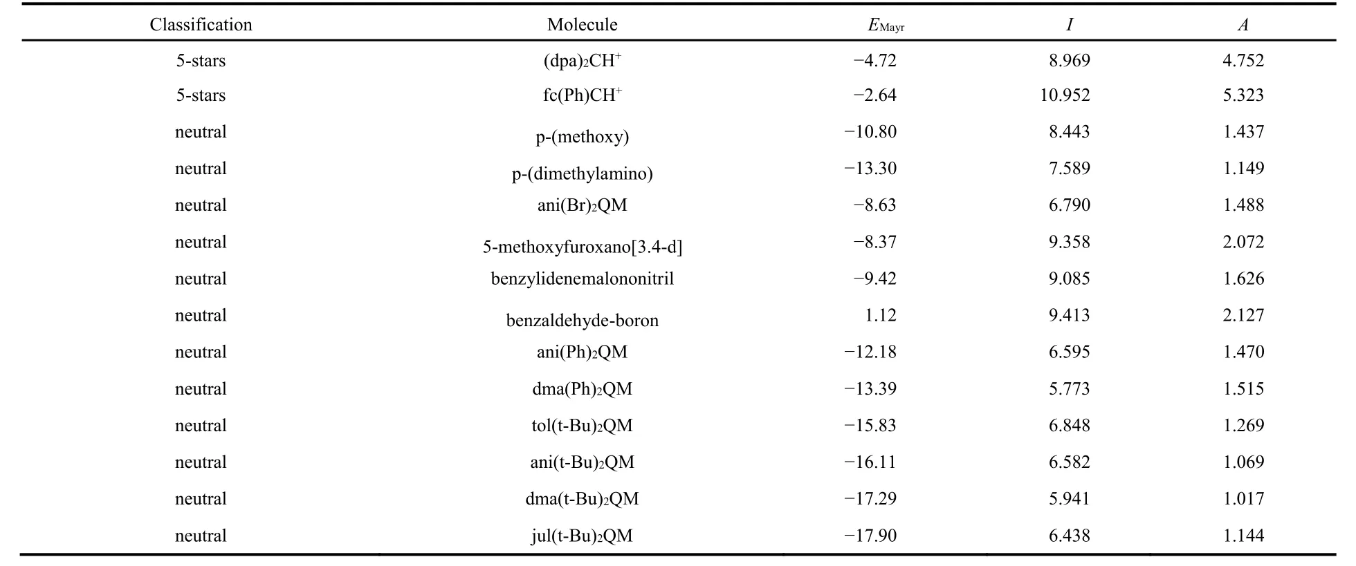
continued Table 1

The SR calculations were performed using GP and GE algorithms, with different “tree lengths”. The mutation probability was set to 15%, and the maximum number of generations was set to 50. For each case, three runs were performed, as a way to check the stability of the SR results. The final expressions were simplified, when possible. These calculations were performed using the HeuristicLab-3.3.12 software package116.

5 Results

5.1 Conceptual DFT results

In Table 2 we show the values of the fitted parameters for every tested model. We have performed 5 different fits, one for each of the 4 separate families of compounds, and one that takes into account all the molecules. It is interesting to note that in the case of the 1-star family the slope of the linear regression(cf. Eq. (24)) is negative when we use the ωparabolic, ωTD, and Pω～ indices. This is a surprising result since these are precisely the electrophilicity measures that have the strongest theoretical justification. This implies that these indices can even give qualitatively wrong results, namely, they are in some cases incapable of predicting the relative order of electrophilicity observed experimentally. This is a reminder that these simple electronic structure-based indices miss many of the factors that govern the tendency of a system to gain electrons during the course of an actual chemical reaction. Nonetheless, it is reassuring that when we work with bigger datasets, all the studied models have positive slopes. This means that, overall,these indices are able to recover the rough trends in Mayr’s electrophilicity parameter.

With the parameters given in Table 1, it is easy to evaluate the quality of the different fits (see Table 3). In general, good correlations are obtained in all cases, with the exception of the 3-stars family. This is probably because the 3-star family is themost structurally diverse group. For example, here we can find heterosubstituted carbocations (like flavylium and 1,3-dithianylium), methal-stabilized carbocations (like the 1,3-diphenylpropyn-1-ylium-Cr(CO)3), benzhydril cations (like pop(tol)CH+and (pfp)2CH+), cyclic conjugated carbocations(like the tropylium ion), and other π-delocalized carbocations(like 1,1,3-triphenylallylium and 1-(4-chlorophenyl) cyclopent-2-enylium). In this case, even the best fit (given by ωTD) still results in an RMSD of 2.950, and a correlation coefficient lower than 0.6. This is a strong indication that to predict the electrophilicity of a given compound we should use a model trained on a set of molecules with similar characteristics. An alternative, in the case we are especially interested in structurally diverse sets, could be to include information regarding condensed local reactivity descriptors117–120.

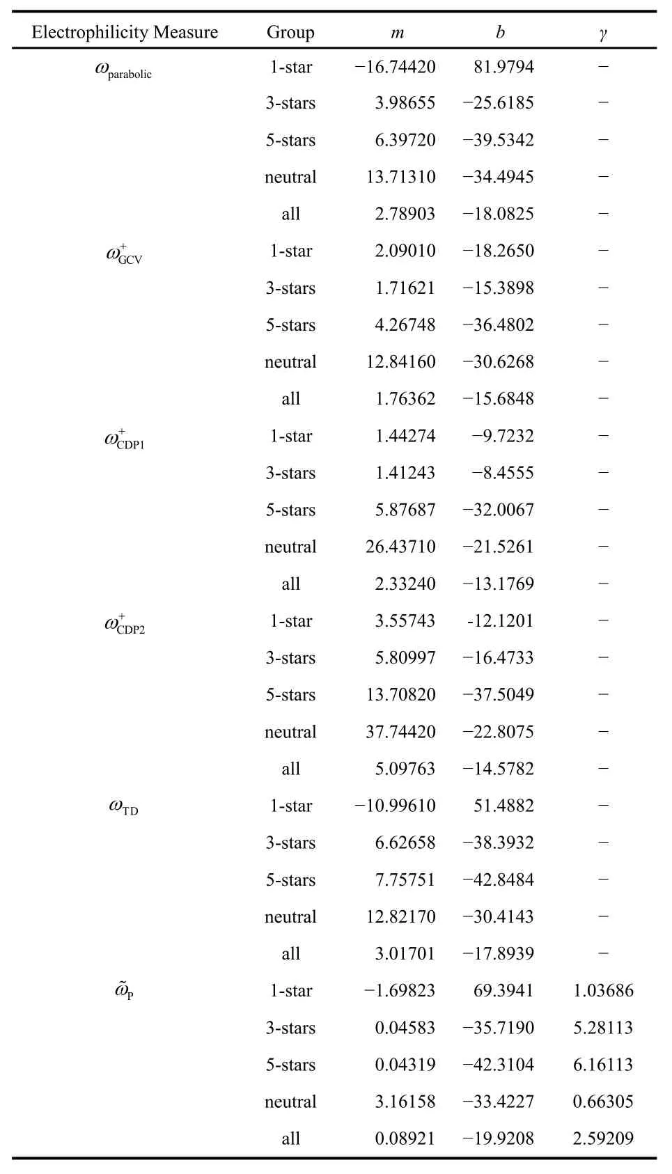
Table 2 Fit parameters for all the c-DFT-based electrophilicity measures studied.

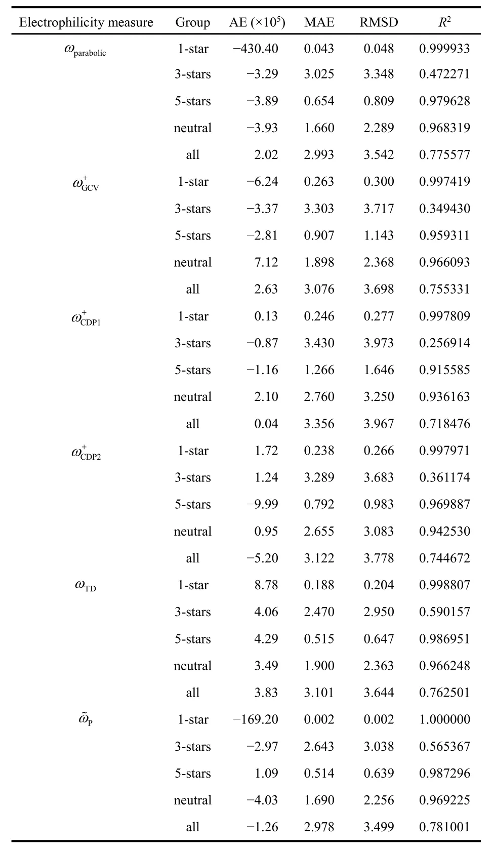
Table 3 Average error (AE), mean absolute error (MAE), root mean square deviation (RMSD), and correlation coefficient (R2) for all the c-DFT-based electrophilicity measures studied.

This insight is supported by the very good fits obtained for the 5-stars and neutral groups (particularly, when we consider the values of R2). These families are mostly formed by structurally similar compounds: benzhydryl cations in the 5-star case, and quinone methides (with a few alkenes substituted with electron-withdrawing groups) in the neutral case. The structural variety of the neutral family is reflected instead in the RMSD values, which are significantly higher than those found in the 5-star case. Overall, all the electrophilicity measures studied have very similar performances over these sets.Nonetheless, in terms of RMSD and R2, the ω+CDP1 and ω+CDP2 indices are outperformed by others. These trends are preserved when we perform the fits including all the studied molecules.Finally, we should note that the simple model based on ωTDconsistently ranks among the best. Recall that is simply equal to the electron affinity; it is not surprising that the electrophilicity and the electron affinity are closely related.

5.2 SR results

In Tables 4 and 5 we show the expressions obtained using GE and GP for all families, respectively. In cases where the optimization algorithm resulted in more than one expression,we will only consider the two that have the highest correlation coefficient values. All the solutions with tree lengths up to 4 are explicitly presented. Additionally, we will also discuss some examples of more complex expressions obtained with greater tree lengths.

Unsurprisingly, given the choice to select between I or A to construct a function to fit EMayr, both algorithms choose the latter. However, here we see much more general functional forms including the electron affinity. For example, now we have a greater variety of terms with different powers of A(ranging from −1 to +3). In all these cases (except in the pathological 1-star family), the final equations are monotonically increasing functions of A.

The results of the different statistical measures corresponding to the SR fits can be found in Table 6. Overall,the performance of these methods is very similar to the c-DFT electrophilicity measures. For example, for the 3-stars family,the RMSD and R2values obtained both by GE and GP algorithms are virtually identical to those corresponding to the best c-DFT indices (ωTDandPω～). For this family, the quality of the fit remains essentially unaltered if we increase the tree length using the GE algorithm (increasing the tree length up to 7 only increases R2up to 0.539182). On the other hand,increasing the tree length does improve the fit quality when we use GP. In this case, a tree length of 7 gave an R2of 0.703165.The corresponding expression (which, in our notation, would be equation gp_73a) is:·

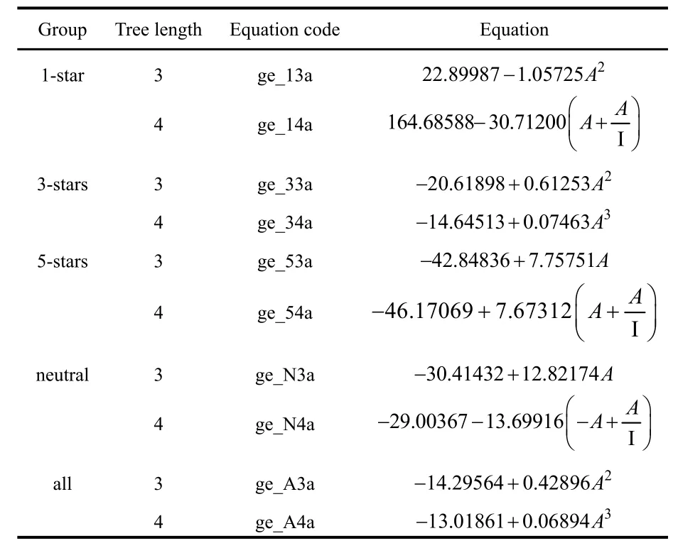
Table 4 Equations obtained using grammatical evolution.

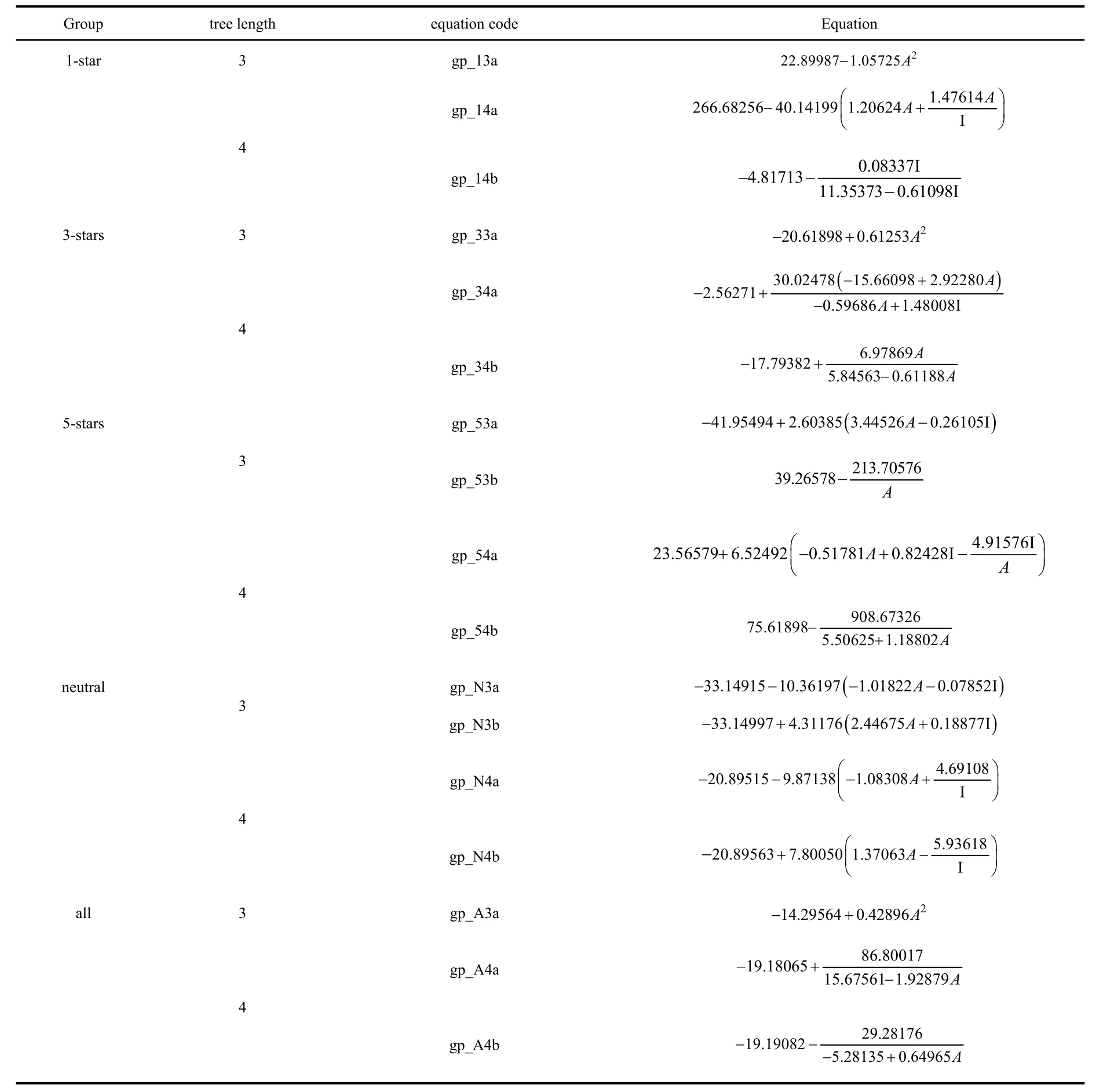
Table 5 Equations obtained using genetic programming.

Nonetheless, requiring an extremely complicated expression to get a semi-quantitative fit is a reminder of the difficulty of predicting experimental electrophilicities with a single expression over a structurally diverse set of compounds.

For the 5-stars family the SR results are excellent, and increasing the tree length in the latter case does not produce a noticeable improvement in the quality of the fit. On the other hand, it is interesting to note that when we work with all the molecules at the same time, the c-DFT indices perform slightly better than the SR expressions. However, when we increase the tree length both GP and GE algorithms provide significantly better solutions. For example, the equation ge_A7a would be:

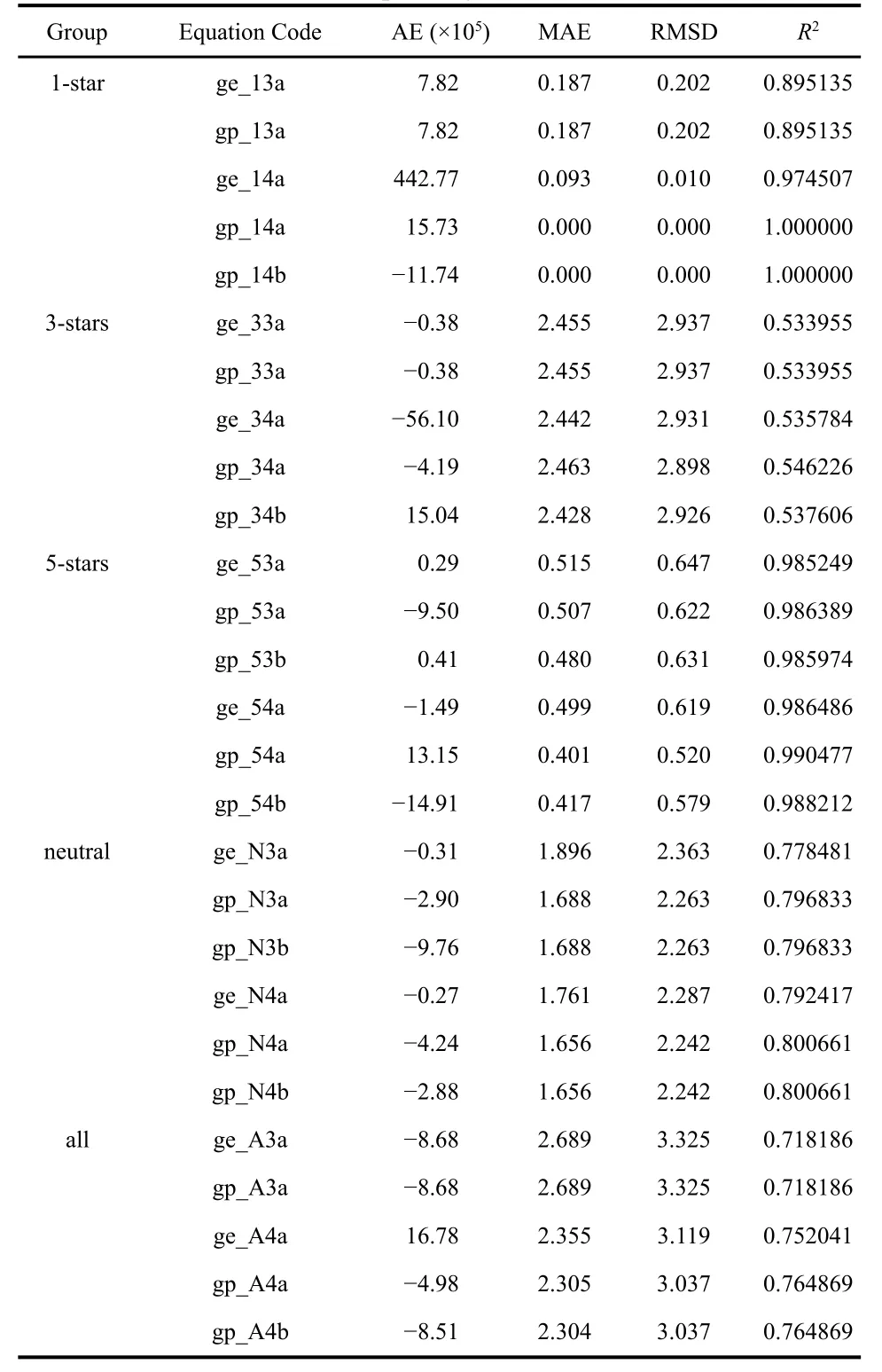
Table 6 Average error (AE), mean absolute error (MAE), root mean square deviation (RMSD), and correlation coefficient (R2) for all the SR-based electrophilicity measures studied.

and it corresponds to an R2of 0.85897. Its GP analog, namely,equation gp_A7a is:

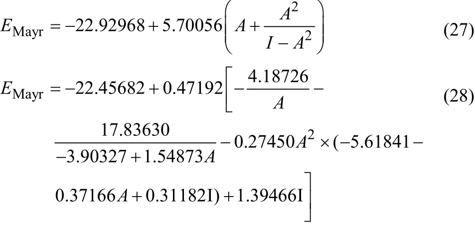
which in turn has an R2of 0.87667.

These results indicate that we need to increase the flexibility of SR methods when the complexity of the system under study increases. This is to be expected since these methods need to“learn” the physical insights that are already built in the c-DFT descriptors.

6 Conclusions

In this work we have assessed how different theoretical electrophilicity measures can be used to predict the experimental values of this index determined by Mayr et al.The different c-DFT indices used provided acceptable results,as long as they were applied to molecules with similar structures. From a quantitative point of view, it is reassuring that a measure as simple as the electron affinity, ωTD, provides results of comparable (if not better) quality than models based on more complex indices. This means that we can predict experimental electrophilicity values without computing the ionization energy, which reduces the computational effort.

Perhaps the biggest appealing of the c-DFT approach is that one uses simple expressions, with chemically-motivated terms.In this way, we gain valuable insights into the factors that determinate the electrophilicity at a molecular level. However,we noticed that there are cases when the c-DFT measures were unable to provide the correct qualitative ordering corresponding to the experimental electrophilicity. This serves as an indication that still more effort is needed to improve the c-DFT descriptors, so they can provide a more realistic description of the electron uptake processes. For example, local reactivity indicators are probably needed in order to compare the electrophilicities of diverse families of molecules that include several different types of electrophilic reactive sites (A similar observation has been made for quantitative studies of the quality of leaving groups28).

To the best of our knowledge, we are reporting the first application of symbolic regression techniques to the prediction of experimental electrophilicity values and the first study of symbolic regression within the conceptual DFT framework.Symbolic regression has the advantage that the resulting models can be improved systematically, by removing restrictions from the optimization process. We showed that this is a key factor for making adequate predictions over relatively complex sets. The simplest models once again proved that the best way to predict the electrophilicity, which often only requires calculating the electron affinity. In general, the expressions obtained using GE are simpler than those obtained using GP, but in most cases the corresponding fits are equivalent. Finally, it should be remarked that, while attractive,these models could be prone to overfitting.

In general, when used carefully, the different theoretical methods studied here provide adequate predictions of the experimental electrophilicity. Further studies are necessary,however, to assess their utility over a broader range of compounds, including their validation using independent “test”sets of molecules. It is also interesting to check whether using the exact electrophilicity formula given in Eq. (19) will improve the quantitative predictions.

(1) Miller, B. Advanced Organic Chemistry: Reactions and Mechanisms;Prentice-Hall: Upper Saddle River, NJ, USA, 1998.doi: 10.1021/ed075p1558

(2) March, J. Advanced Organic Chemistry; Wiley-Interscience: New York, NY, USA, 1992. doi: 10.1002/0470084960

(3) Mayr, H.; Kempf, B.; Ofial, A. R. Acc. Chem. Res. 2003, 36, 66.doi: 10.1021/ar020094c

(4) Mayr, H.; Bug, T.; Gotta, M. F.; Hering, N.; Irrgang, B.; Janker, B.;Kempf, B.; Loos, R.; Ofial, A. R.; Remennikov, G.; et al. J. Am.Chem. Soc. 2001, 123, 9500. doi: 10.1021/ja010890y

(5) Mayr, H.; Patz, M. Angew. Chem. Int. Ed. 1994, 33, 938.doi: 10.1002/anie.199409381

(6) Mayr, H.; Ofial, A. R. J. Phys. Org. Chem. 2008, 21, 584.doi: 10.1002/poc.1325

(7) Mayr, H.; Ofial, A. R. Pure Appl. Chem. 2005, 77, 1807.doi: 10.1351/pac200577111807

(8) Liu, S. B. In Chemical Reactivity Theory: A Density Functional View; Chattaraj, P. K., Ed.; Taylor and Francis: Boca Raton, FL,USA, 2009; p. 179.

(9) Chattaraj, P. K.; Giri, S. Ann. Rep. Prog. Chem. C 2009, 105, 13.doi: 10.1039/B802832J

(10) Chattaraj, P. K.; Giri, S.; Duley, S. Chem. Rev. 2011, 111, PR43.doi: 10.1021/cr100149p

(11) Maynard, A. T.; Huang, M.; Rice, W. G.; Covell, D. G. Proc. Natl.Acad. Sci. USA 1998, 95, 11578. doi: 10.1073/pnas.95.20.11578

(12) Parr, R. G.; von Szentpály, L.; Liu, S. B. J. Am. Chem. Soc. 1999,121, 1922. doi: 10.1021/ja983494x

(13) Chermette, H. J. Comput. Chem. 1999, 20, 129.doi: 10.1002/(SICI)1096-987X(19990115)20:1＜129::AID-JCC13＞3.0.CO;2-A

(14) Parr, R. G.; Yang, W. Density-Functional Theory of Atoms and Molecules; Oxford UP: New York, NY, USA, 1989.

(15) Geerlings, P.; De Proft, F.; Langenaeker, W. Chem. Rev. 2003, 103,1793. doi: 10.1021/cr990029

(16) Johnson, P. A.; Bartolotti, L. J.; Ayers, P. W.; Fievez, T.; Geerlings,P. Modern Charge Density Analysis; Gatti, C., Macchi, P., Eds.;Springer: New York, NY, USA, 2012; p. 715.

(17) Ayers, P. W.; Anderson, J. S. M.; Bartolotti, L. J. Int. J. Quantum Chem. 2005, 101, 520. doi: 10.1002/qua.20307

(18) Ayers, P. W.; Parr, R. G. J. Am. Chem. Soc. 2000, 122, 2010.doi: 10.1021/ja9924039

(19) Miranda-Quintana, R. A. Conceptual Density Functional Theory and its Applications in the Chemical Domain; Islam, N., Kaya, S., Eds.;Apple Academic Press: NJ, USA, in press.

(20) Chemical Reactivity Theory: A Density Functional View; Chattaraj,P. K., Ed.; CRC Press: Boca Raton, FL, USA, 2009.

(21) Fuentealba, P.; Cárdenas, C. Chemical Modelling; Springborg, M.,Ed.; The Royal Society of Chemistry: London, UK, 2015; Vol. 11, p.151.

(22) Liu, S. B. Acta Phys. -Chim. Sin. 2009, 25, 590.doi: 10.3866/PKU.WHXB20090332

(23) Gazquez, J. L. J. Mex. Chem. Soc. 2008, 52, 3.

(24) Domingo, L. R.; Perez, P.; Saez, J. A. RSC Adv. 2013, 3, 1486.doi: 10.1039/C2RA22886F

(25) Domingo, L. R.; Zaragoza, R. J.; Saez, J. A.; Arno, M. Molecules 2012, 17, 1335. doi: 10.3390/molecules17021335

(26) Domingo, L. R.; Perez, P.; Contreras, R. Tetrahedron 2004, 60,6585. doi: 10.1016/j.tet.2004.06.003

(27) Domingo, L. R.; Aurell, M. J.; Perez, P.; Contreras, R. J. Phys.Chem. A 2002, 106, 6871. doi: 10.1021/jp020715j

(28) Anderson, J. S. M.; Liu, Y. L.; Thomson, J. W.; Ayers, P. W. J. Mol.Struct.: THEOCHEM 2010, 943, 168.doi: 10.1016/j.theochem.2009.12.013

(29) Ayers, P. W.; Anderson, J. S. M.; Rodriguez, J. I.; Jawed, Z. Phys.Chem. Chem. Phys. 2005, 7, 1918. doi: 10.1039/B500996K

(30) Chamorro, E.; Chattaraj, P. K.; Fuentealba, P. J. Phys. Chem. A 2003, 107, 7068. doi: 10.1021/jp035435y

(31) Parthasarathi, R.; Elango, M.; Subramanian, V.; Chattaraj, P. K.Theor. Chem. Acc. 2005, 113, 257. doi: 10.1007/s00214-005-0634-3

(32) González, M. M.; Hernández-Castillo, D.; Montero-Cabrera, L. A.;Miranda-Quintana, R. A. Int. J. Quantum Chem. 2017, e25444.doi: 10.1002/qua.25444

(33) Moens, J.; Jaque, P.; De Proft, F.; Geerlings, P. J. Phys. Chem. A 2008, 112, 6023. doi: 10.1021/jp711652a

(34) Moens, J.; Geerlings, P.; Roos, G. Chem. -A Eur. J. 2007, 13, 8174.doi: 10.1002/chem.200601896

(35) Moens, J.; Roos, G.; Jaque, P.; Proft, F.; Geerlings, P. Chem. -A Eur.J. 2007, 13, 9331. doi: 10.1002/chem.200700547

(36) Parthasarathi, R.; Padmanabhan, J.; Subramanian, V.; Maiti, B.;Chattaraj, P. K. Curr. Sci. 2004, 86, 535.

(37) Parthasarathi, R.; Subramanian, V.; Roy, D. R.; Chattaraj, P. K.Biorg. Med. Chem. 2004, 12, 5533. doi: 10.1016/j.bmc.2004.08.013

(38) Rétey, J. Biochim. Biophys. Acta 2003, 1647, 179.doi: 10.1016/S1570-9639(03)00091-8

(39) Rosenkranz, H. S.; Klopman, G.; Zhang, Y.; Graham, C.; Karol, M.H. Environ. Health Perspect. 1999, 107, 129.

(40) Miranda-Quintana, R. A. J. Chem. Phys. 2017, 146, 046101.doi: 10.1063/1.4974987

(41) Pan, S.; Sola, M.; Chattaraj, P. K. J. Phys. Chem. A 2013, 117, 1843.doi: 10.1021/jp312750n

(42) Morell, C.; Labet, V.; Grand, A.; Chermette, H. Phys. Chem. Chem.Phys. 2009, 11, 3414. doi: 10.1039/B818534D

(43) Chattaraj, P. K. Indian J. Phys. Proc. Indian Assoc. Cultiv. Sci. 2007,81, 871

(44) Miranda-Quintana, R. A.; Chattaraj, P. K.; Ayers, P. W. J. Chem.Phys. 2017, 147, 124103. doi: 10.1063/1.4996443

(45) Gazquez, J. L.; Cedillo, A.; Vela, A. J. Phys. Chem. A 2007, 111,1966. doi: 10.1021/jp065459f

(46) Chamorro, E.; Duque-Noreña, M.; Perez, P. J. Mol. Struct. 2009,896, 73. doi: 10.1016/j.theochem.2008.11.009

(47) Chamorro, E.; Duque-Noreña, M.; Perez, P. J. Mol. Struct. 2009,901, 145. doi: 10.1016/j.theochem.2009.01.014

(48) Franco-Pérez, M.; Gazquez, J. L.; Ayers, P. W. Acta Phys. -Chim.Sin. 2018, submitted.

(49) Miranda-Quintana, R. A. J. Chem. Phys. 2017, 146, 214113.doi: 10.1063/1.4984611

(50) Parr, R. G.; Pearson, R. G. J. Am. Chem. Soc. 1983, 105, 7512.doi: 10.1021/ja00364a005

(51) Parr, R. G.; Donnelly, R. A.; Levy, M.; Palke, W. E. J. Chem. Phys.1978, 68, 3801. doi: 10.1063/1.436185

(52) Sanderson, R. T. Science 1951, 114, 670.doi: 10.1126/science.114.2973.670

(53) Galvan, M.; Vela, A.; Gazquez, J. L. J. Phys. Chem. 1988, 92, 6470.doi: 10.1021/j100333a056

(54) Vargas, R.; Galvan, M.; Vela, A. J. Phys. Chem. A 1998, 102, 3134.doi: 10.1021/jp972984t

(55) Galvan, M.; Vargas, R. J. Phys. Chem. 1992, 96, 1625.doi: 10.1021/j100183a026

(56) Ghanty, T. K.; Ghosh, S. K. J. Am. Chem. Soc. 1994, 116, 3943.doi: 10.1021/ja00088a033

(57) Chamorro, E.; Santos, J. C.; Escobar, C. A.; Perez, P. Chem. Phys.Lett. 2006, 431, 210. doi: 10.1016/j.cplett.2006.09.072

(58) Chamorro, E.; Perez, P.; De Proft, F.; Geerlings, P. J. Chem. Phys.2006, 124, 044105. doi: 10.1063/1.2161187

(59) Perez, P.; Chamorro, E.; Ayers, P. W. J. Chem. Phys. 2008, 128,204108. doi: 10.1063/1.2916714

(60) Miranda-Quintana, R. A.; Ayers, P. W. Theor. Chem. Acc. 2016,135, 239. doi: 10.1007/s00214-016-1995-5

(61) Cardenas, C.; Heidar Zadeh, F.; Ayers, P. W. Phys. Chem. Chem.Phys. 2016, 18, 25721. doi: 10.1039/C6CP04533B

(62) Perdew, J. P.; Parr, R. G.; Levy, M.; Balduz, J. L., Jr. Phys. Rev. Lett.1982, 49, 1691. doi: 10.1103/PhysRevLett.49.1691

(63) Heidar Zadeh, F.; Miranda-Quintana, R. A.; Verstraelen, T.;Bultinck, P.; Ayers, P. W. J. Chem. Theory Comp. 2016, 12, 5777.doi: 10.1021/acs.jctc.6b00494

(64) Miranda-Quintana, R. A.; Ayers, P. W. Conceptual Density Functional Theory and Its Applications in the Chemical Domain;Islam, N., Kaya, S., Eds.; Apple Academic Press: NJ, USA, in press.

(65) Miranda-Quintana, R. A.; Ayers, P. W. J. Chem. Phys. 2016, 144,244112. doi: 10.1063/1.4953557

(66) Ayers, P. W.; Parr, R. G. J. Chem. Phys. 2008, 129, 054111.doi: 10.1063/1.2957900

(67) Ayers, P. W.; Parr, R. G. J. Chem. Phys. 2008, 128, 184108.doi: 10.1063/1.2918731

(68) Franco-Pérez, M.; Ayers, P. W.; Gazquez, J. L.; Vela, A. J. Chem.Phys. 2017, 147, 094105. doi: 10.1063/1.4999761

(69) Franco-Pérez, M.; Heidar-Zadeh, F.; Ayers, P. W.; Gazquez, J. L.;Vela, A. Phys. Chem. Chem. Phys. 2017, 19, 11588.doi: 10.1039/C7CP00224F

(70) Franco-Pérez, M.; Ayers, P. W.; Gazquez, J. L.; Vela, A. Phys.Chem. Chem. Phys. 2017, 19, 13687. doi: 10.1039/C7CP00692F

(71) Polanco-Ramírez, C. A.; Franco-Pérez, M.; Carmona-Espíndola, J.;Gazquez, J. L.; Ayers, P. W. Phys. Chem. Chem. Phys. 2017, 19,12355. doi: 10.1039/C7CP00691H

(72) Franco-Pérez, M.; Ayers, P.; Gazquez, J. L.; Vela, A. J. Chem. Phys.2015, 143, 244117. doi: 10.1063/1.4938422

(73) Franco-Pérez, M.; Gazquez, J. L.; Ayers, P.; Vela, A. J. Chem. Phys.2015, 143, 154103. doi: 10.1063/1.4932539

(74) Malek, A.; Balawender, R. J. Chem. Phys. 2015, 142, 054104.doi: 10.1063/1.4906555

(75) Miranda-Quintana, R. A.; Ayers, P. W. Phys. Chem. Chem. Phys.2016, 18, 15070. doi: 10.1039/c6cp00939e

(76) Miranda-Quintana, R. A. Theor. Chem. Acc. 2017, 136, 76.doi: 10.1007/s00214-017-2109-8

(77) Miranda-Quintana, R. A.; Ayers, P. W. Theor. Chem. Acc. 2016,135, 172. doi: 10.1007/s00214-016-1924-7

(78) Miranda-Quintana, R. A. Theor. Chem. Acc. 2016, 135, 189.doi: 10.1007/s00214-016-1945-2

(79) Miranda-Quintana, R. A.; González, M. M.; Ayers, P. W. Phys.Chem. Chem. Phys. 2016, 18, 22235. doi: 10.1039/c6cp03213c

(80) Klopman, G. J. Am. Chem. Soc. 1968, 90, 223.doi: 10.1021/ja01004a002

(81) Klopman, G.; Hudson, R. F. Theor. Chim. Act. 1967, 8, 165.doi: 10.1007/bf00526373

(82) Klopman, G.; Klopman, G. Chemical Reactivity and Reaction Paths;Wiley-Interscience: New York, NY, USA, 1974; p. 55.

(83) Hudson, R. F.; Klopman, G. Tetrahedron Lett. 1967, 12, 1103.doi: 10.1016/S0040-4039(00)90645-2

(84) Salem, L. J. Am. Chem. Soc. 1968, 90, 553.doi: 10.1021/ja01005a002

(85) Salem, L. J. Am. Chem. Soc. 1968, 90, 543.doi: 10.1021/ja01005a001

(86) Salem, L. Chem. Br. 1969, 5, 449.

(87) Witten, I. H.; Frank, E.; Hall, M. A.; Pal, C. J. Data Mining:Practical Machine Learning Tools and Techniques, 4th ed.; Elsevier:Cambridge, MA, USA, 2017.

(88) Gertrudes, J. C.; Maltarollo, V. G.; Silva, R. A.; Oliveira, P. R.;Honorio, K. M.; da Silva, A. B. F. Curr. Med. Chem. 2012, 19, 4289.doi: 10.2174/092986712802884259

(89) Carrera, G.; Gupta, S.; Aires-de-Sousa, J. J. Comput. Aided Mol.Des. 2009, 23, 419. doi: 10.1007/s10822-009-9275-2

(90) Dietterich, T. G. Ai Mag. 1997, 18, 97.doi: 10.1609/aimag.v18i4.1324

(91) Carbonell, J. G.; Michalski, R. S.; Mitchell, T. M. Machine Learning: an Artificial Intelligence Approach; Michalski, R. S.,Carbonell, J. G., Mitchell, T. M., Eds.; Springer Berlin Heidelberg:Berlin, Heidelberg, Germany, 1983; p. 3.doi: 10.1007/978-3-662-12405-5_1

(92) Lino, A.; Rocha, A.; Sizo, A. J. Intell. Fuzzy Syst. 2016, 31, 2061.doi: 10.3233/JIFS-169045

(93) Affenzeller, M.; Winkler, S. M.; Kronberger, G.; Kommenda, M.;Burlacu, B.; Wagner, S. Genetic Programming Theory and Practice XI; Riolo, R., Moore, J. H., Kotanchek, M., Eds.; Springer New York: New York, NY, USA, 2014; p. 175.doi: 10.1007/978-1-4939-0375-7_10

(94) Billard, L.; Diday, E. Classification, Clustering, and Data Analysis:Recent Advances and Applications; Jajuga, K., Sokolowski, A.,Bock, H. H., Eds.; Springer-Verlag: Berlin, Germany, 2012.

(95) Billard, L.; Diday, E. J. Am. Stat. Assoc. 2003, 98, 470.doi: 10.1198/016214503000242

(96) Billard, L.; Diday, E. Data Analysis, Classification, and Related Methods; Kiers, H. A. L., Rasson, J.-P., Groenen, P. J. F., Schader,M., Eds.; Springer Berlin Heidelberg: Berlin, Heidelberg, Germany,2000; p. 369. doi: 10.1007/978-3-642-59789-3_58

(97) Schmidt, M. D.; Vallabhajosyula, R. R.; Jenkins, J. W.; Hood, J. E.;Soni, A. S.; Wikswo, J. P.; Lipson, H. Phys. Biol. 2011, 8, 055011.doi: 10.1088/1478-3975/8/5/055011

(98) Schmidt, M. W.; Lipson, H. Science 2009, 324, 81.doi: 10.1126/science.1165893

(99) Bongard, J.; Lipson, H. Proc. Natl. Acad. Sci. USA 2007, 104, 9943.doi: 10.1073/pnas.0609476104

(100) Quade, M.; Abel, M.; Shafi, K.; Niven, R. K. Phys. Rev. B 2016, 94,012214. doi: 10.1103/PhysRevE.94.012214

(101) Koza, J. R. 2nd International IEEE Conference on Tools for Artificial Intelligence, 1990; p. 819.

(102) Sharma, S.; Tambe, S. S. Biochem. Eng. J. 2014, 85, 89.doi: 10.1016/j.bej.2014.02.007

(103) Langdon, W. B.; Poli, R. Found. Genet. Program.; Springer-Verlag:Berlin, Germany, 2013.

(104) O’Neil, M.; Ryan, C. Grammatical Evolution: Evolutionary Automatic Programming in an Arbitrary Language; Springer US:Boston, MA, USA, 2003; p. 33. doi: 10.1007/978-1-4615-0447-4_4

(105) O’Neil, M.; Ryan, C. Grammatical Evolution: Evolutionary Automatic Programming in an Arbitrary Language; Springer US:Boston, MA, USA, 2003; p. 79. doi: 10.1007/978-1-4615-0447-4_7

(106) Ryan, C.; Collins, J.; Neill, M. O. Genetic Programming: First European Workshop, EuroGP’98 Paris, France, April 14–15, 1998 Proceedings; Banzhaf, W., Poli, R., Schoenauer, M., Fogarty, T. C.,Eds.; Springer: Berlin, Heidelberg, Germany, 1998;, p. 83.doi: 10.1007/BFb0055930

(107) Luke, S.; Spector, L. Genetic Programming 1997: Proceedings of the Second Annual Conference (GP97); Koza, J., Ed.; San Francisco,CA, USA, 1997; p. 240.

(108) Spears, W. M.; Anand, V. Methodologies for Intelligent Systems: 6th International Symposium, ISMIS '91 Charlotte, N. C., USA, October 16–19, 1991 Proceedings; Ras, Z. W., Zemankova, M., Eds.;Springer: Berlin, Heidelberg, Germany, 1991; p. 409.doi: 10.1007/3-540-54563-8_104

(109) Chomsky, N. IRE Trans. Inf. Theory 1956, 2, 113.doi: 10.1109/TIT.1956.1056813

(110) Ginsburg, S. The Mathematical Theory of Context Free Languages;McGraw-Hill, New York, NY, USA, 1966.

(111) Temkin, J. M.; Gilder, M. R. Bioinformatics 2003, 19, 2046.doi: 10.1093/bioinformatics/btg279

(112) Trelea, I. C. Inf. Proc. Lett. 2003, 85, 317.doi: 10.1016/S0020-0190(02)00447-7

(113) Mayr, H. http://www.cup.lmu.de/oc/mayr/reaktionsdatenbank/; Vol.2017 (accessed Oct 30, 2017).

(114) Mayr, H. http://www.cup.uni-muenchen.de/oc/mayr/DBintro.html;Vol. 2017 (accessed Oct 30, 2017).

(115) Frisch, M. J.; Trucks, G. W.; Schlegel, H. B.; Scuseria, G. E.; Robb,M. A.; Cheeseman, J. R.; Scalmani, G.; Barone, V.; Mennucci, B.;Petersson, G. A.; et al. Gaussian 09; Gaussian Inc.: Wallingford, CT,USA, 2009.

(116) Wagner, S.; Kronberger, G.; Beham, A.; Kommenda, M.;Scheibenpflug, A.; Pitzer, E.; Vonolfen, S.; Kofler, M.; Winkler, S.;Dorfer, V.; et al. Advanced Methods and Applications in Computational Intelligence; Klempous, R., Nikodem, J., Jacak, W.,Chaczko, Z., Eds.; Springer International Publishing: Heidelberg,Germany, 2014; p. 197. doi: 10.1007/978-3-319-01436-4_10

(117) Yang, W. T.; Mortier, W. J. J. Am. Chem. Soc. 1986, 108, 5708.doi: 10.1021/ja00279a008

(118) Miranda-Quintana, R. A. Chem. Phys. Lett. 2016, 658, 328.doi: 10.1016/j.cplett.2016.06.068

(119) Zielinski, F.; Tognetti, V.; Joubert, L. Chem. Phys. Lett. 2012, 527,67. doi: 10.1016/j.cplett.2012.01.011

(120) Bultinck, P.; Fias, S.; Alsenoy, C. V.; Ayers, P. W.; Carbó-Dorca, R.J. Chem. Phys. 2007, 127, 034102. doi: 10.1063/1.2749518