Software Defect Distribution Prediction Model Based on NPE-SVM
2018-06-07HuaWeiChunShanChangzhenHuHuizhongSunMinLei5
Hua Wei, Chun Shan, Changzhen Hu, Huizhong Sun*, Min Lei5
1 School of Computer Science and Technology, Beijing Institute of Technology, Beijing 100081, China
2 China Information Technology Security Evaluation Center, Beijing 100085, China
3 Beijing Key Laboratory of Software Security Engineering Technology, School of Software, Beijing Institute of Technology,Beijing 100081, China
4 Information Security Center, Beijing University of Posts and Telecommunications, Beijing 100876, China
5 Guizhou University, Guizhou Provincial Key Laboratory of Public Big Data, Guizhou Guiyang 550025, China
I. INTRODUCTION
In recent years, the technology of machine learning developed so rapidly and has been widely used in many research fields, including the predictions of the software defect distribution [1][2][3][4][5]. Software defect distribution prediction plays an important role in the whole process of software development.Timely and accurate prediction of defective software modules will greatly improve the effective allocation of software testing resources[6]. There are many researchers has collected many training samples by extracting the software metric attributes of the software modules,and constructed the software defect distribution prediction model by employing different kinds of machine learning technology. The machine learning technology has been introduced to the field of software defect prediction in [7][8]. David Bowes et al.[9] performed a sensitivity analysis to compare the performance of different algorithms, e.g., Random Forest, Naive Bayes, RPart and SVM classifiers, when predicting defects in NASA, open source and commercial datasets. Yongquan Yan et al.[10] proposed a method which can give practice guide to forecast software aging using machine learning algorithm.Liqiang Zhang et al.[11] present a measurement framework for evaluating these metrics.Zibin Zheng et al. [12] proposed a research framework for predicting reliability of individual software entities as well as the whole Internet application.Pengcheng Zhang et al.[13] proposed a novel Bayesian combinational model to predict QoS by continuously adjusting credit values of the basic models so as to keep good prediction accuracy. ChengshengYuan et al.[14] proposed a new software-based liveness detection approach using multi-scale local phase quantity (LPQ) and principal component analysis(PCA) . Yiqi Fu et al.[15] conducted comparative analysis to different machine learning based defect prediction methods, and found that different algorithms have both advantages and disadvantages in different evaluation tasks. Malhotra et al.[16] assessed the performance capability of the machine learning techniques in existing research for software fault prediction. They compared the performance of the machine learning techniques with the statistical techniques and other machine learning techniques.
In this paper, the authors proposed an improved NPE-SVM software defect prediction model based on NPE algorithm,which is one kind of the manifold learning algorithm.
However, all the above research methods do not consider two practical problems in software defect prediction. Firstly, there is a serious problems of class imbalance in the software defect data. Boehm pointed out that 20 percent of software modules in software systems contain 80 percent of software defects[17]. In other words, most of the software defects appear in a few software modules. Secondly, it is costly to collect a large amount of training data with labels. In practice, it takes a lot of time, manpower and other test resources,and even that expert knowledge is needed to collect the training data with labels. Moreover,it is almost unrealistic to obtain large quantities of labeled sample data for those projects without historical versions [18]. This poses a great challenge to the existing supervised forecasting model. It is difficult to construct an ideal classifier with a small quantity of defect training data. In this paper, we proposes a software defect distribution prediction model based on the improved NPE-SVM algorithm.The main contributions include the following three aspects:
(1) The improved NPE algorithm tackles the central difficulties of software defect measurement in high-dimensional and small sample cases i.e., the analyses of singular matrix of the generalized characteristic matrix and the completeness and robustness of the solution. By using the matrix analysis method,the solution can be effectively processed and effectively applied in the practical application which does not significantly increase the complexity of the algorithm, and result in no loss of useful information.
(2) The improved NPE algorithm transforms the singular generalized eigenvalue problem in the NPE method, i.e., singular generalized eigensystem computation, into two feature decomposition problems, i.e.,eigenvalue decomposition and EVD. In this case, the first feature breaks down to simplify the calculation of generalized features without losing useful discriminating information. The second feature is to break down the unstable broad features and convert the problems into stable features.
(3) Based on the intrinsic matrix structure and correlation of software defect data, this paper discusses the learning ability of direct application of traditional manifold learning methods in matrix data representation, and further reduces computational complexity and maintains the structural characteristics of software defect measurement metadata.
In order to predict the various defects in the software more accurately and improve the quality of the software, it is necessary to reduce the dimensionality of the high-dimensional software metric data. Manifold learning is an important method to deal with high-dimensional data, and it can discover the real structure hidden in high-dimensional software metric data. At present, the main method proposed by researchers are the local linear Embedding (LLE) [19], and Isometric Feature Mapping [20]. However, they both have a common defect: only mapping in the training data, not directly mapping these new test data,which leads to the problem of out-of-sample.In this paper, the software defect distribution prediction model based on improved NPESVM is proposed to solve these problems.By adjusting the correlation coefficients between data, the model solves the problem of high-dimensional and small sampling, and then extracts the features of low dimensional data. We compared several nonlinear dimensionality reduction algorithms to extract the in fluence of software defect characteristics on the prediction results. Through experimental verification, we find that the model greatly improves the accuracy of the software defect distribution prediction.
The rest of this paper is organized as follows. Section II presents some related work and our optimized NPE algorithm. In Section III, we describe the NPE-SVM software defect prediction model. In Section IV, we provide a general discussion of commonly used defect prediction techniques and metrics. Finally,Section V gives conclusions and future work.
II. THE NPE ALGORITHM AND ITS IMPROVEMENT
2.1 NPE Algorithm
The main idea of the NPE algorithm is that in the high-dimensional space, each data point is represented by K neighborhood points. After dimensionality reduction, the weights of each nearest neighbor point are kept unchanged,and the reconstructed dimension is simplified by corresponding to the data points, so that the reconstruction error is minimized [21].
Suppose that there is a data setwhere D is the dimension of the observed data, and N is the sample size. The matrix of the front stack is denoted as X=[x1,x2,...,xn]∈RD*N. The essence of linear dimensionality is to find a set of linear projection directions g1,g2,...,gd, and the projection matrix is denoted by G=[g1,g2,...,gd]∈RD*N, such that the low-dimensional embedding identifier yi=GTxiafter projection is the low-dimensional representation of the original data xi.The specific implementation process is as follows:
(1) Finding nearest neighbors points: according to the criteria, a certain number of nearest neighbor points of each data point xiis selected. For example, for each sample point xi, the K nearest distance points are selected as nearest neighbor points, typically based on the Euclidean distance. In the specific application of pattern classification, as the label information of training data is known, so we often use these tags information to assist in selecting nearest neighbor points. If and only if the label information of the two samples is the same and one point is in the K nearest neighbor point of the other one, it can be selected as the nearest neighbor point.
(2) Calculating the optimal reconstruction weight matrix. For each data point Xi, linear reconstruction is performed locally with its nearest neighbor data point Xjby minimizing the reconstruction error for all data points as follows,

The linear reconstruction error function is minimized if the weight matrix W satisfies the sparseness condition wij=0 (Suppose that the j data point does not belong to the nearest neighbor of the i reconstruction data point)and the normalization conditionWe can get the optimal weight matrix.
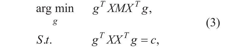
(3) Obtaining the low dimensional embedding representation. In order to maintain the local reconstruction relationship between the samples, the last step of the NPE is to construct the embedded coordinate representation of the data in the d-dimensional Euclidean space, using the reconstructed weight wijof the original high dimensional data space as constraints. The optimization formulation objective function can be expressed as

In the above expression, c is a suitable positive constant which makes g a unit vector.The minimization formula (2) is to ensure that the weights wijthat characterize the primitive space local neighbors relationship are also used to reconstruct the embedded representation of the low-dimensional space. Then,low-dimensional data will still retain some of the local geometry of the original data.
According to simple algebraic deduction,the above formula (2) can be transformed into:
where M = (1-W)T(1-W).
It is not hard to prove that the column vector of the linear projection matrix G is the eigenvector which corresponds to the most minimal d feature values of the following generalized feature problem:

The first two steps of NPE are exactly the same as its nonlinear counterpart LLE algorithm, and they differ from the optimization objective function and constraints.
2.2 Analysis of the problems
In practical applications, the existing observation matrix may lose the part information of the original signal after compressing sampling[22].if the data obtained with high-dimensional and small sampling characteristics,i.e., the data dimension D is high and the number of samples is relatively small and N <<D,then the implementation of NPE algorithm will encounter the following problems:
(1)The dimension of the feature matrix XMXTand XXTis D×D. When D is very large,the dimension of these feature matrices are too large. So it is difficult to calculate the linear transformation by solving spectral decomposition XMXTg =λX XTg of generalized feature matrix, which requires a lot of time and space.
(2) The rank of the feature matrix XXTis rank(XXT)=rank(X)≤min(D,N)=N, where XXTis a matrix of D×D. So in the case of high-dimensional small sampling, XXTis a singular matrix, which further makes the direct implementation of NPE infeasible.
2.3 Improvement of NPE algorithm
In order to solve the above problems, we combine the NPE algorithm with the linear projection direction (3) in the last step of the high-dimensional small sampling case. The following is the specific process of NPE algorithm improvement.
(1) Calculating the eigen-decomposition of matrix
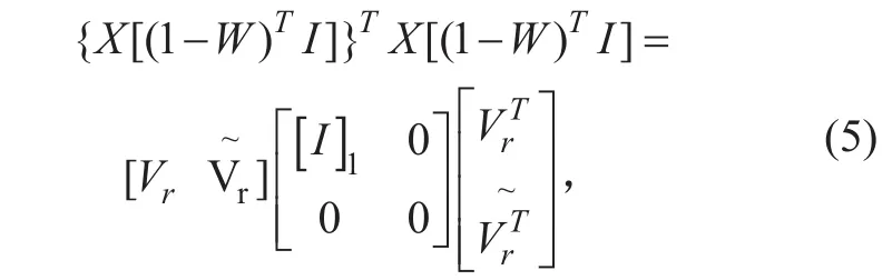
where [I]1is the diagonal proof of the matrix’s non-zero feature values from large to small order, Vr and V~rare composed of eigenvectors corresponding to non-zero feature values and eigenvectors corresponding to zero feature values respectively.
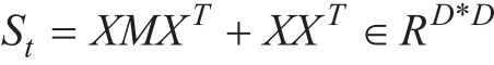
(2)Calculating the matrices Ur and ∑Iin the feature decomposition of the matrix
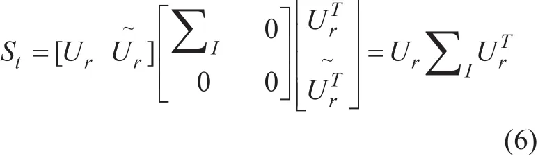
where
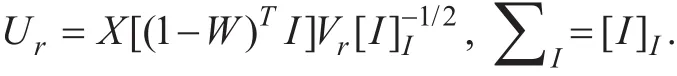
(3) Calculating the eigen-decomposition of matrix

(4) The obtained linear projection matrix G is the former d unit column vector of
The improved NPE algorithm has the following desired features. It solves the singular problem of generalized feature decomposition in high-dimensional small samples, and does not require other intermediate processes to reduce the dimensionality. It can decompose the high-dimensional data effectively, and the resulting feature vectors are more stable and correct, and reduce the computational complexity and computational cost effectively.
III. THE SOFTWARE DEFECT DISTRIBUTION PREDICTION MODEL
3.1 NPE-SVM software defect prediction model
Based on the NPE-SVM algorithm, the software defect distribution prediction model is divided into the following steps:
Step 1: Obtaining the software defect dataset;
Step 2: The training set (Training Set) is selected in the dataset, and the improved NPE algorithm is used to reduce the dimension of the training set;
Step 3: The reduced dimension data obtained from the second step is used as the input dataset of the third step. Since that the radial basis function (RBF) support vector machines (SVM) has the advantage of using a regularization parameter to control the number of support vectors and margin errors in software defect prediction [23].Recently, an interesting accurate on-line algorithm was proposed for training v-support vector classification, which can handle a quadratic formulation with a pair of equality constraints[24].so the kernel function of support vector machine in the model selection uses the RBF function, as shown in (8). According to the defined value interval and the step size, the network search combined with 10-fold cross validation is used to optimize the parameters, and obtain the optimal parameters;

Step 4: Model testing are performed using the optimal parameters obtained in the third step;
Step 5: The software defect pro file prediction is predicted by the reduced dimension dataset. If the prediction result satisfies the terminating condition, the optimized software defect distribution prediction model is obtained and ended. Otherwise, third steps will be continued to optimize the model. In this process,the termination condition is that the prediction accuracy of the model reaches a given threshold or the number of cycles exceeds the maximum number of cycles.
3.2 Parameter selection of NPE-SVM
The NPE-SVM software defect distribution prediction model consists of two parts: improved neighborhood preserving embedding(NPE) and support vector machine (SVM).Support vector ordinal regression (SVOR) is a popular method to tackle ordinal regression problems. In the neighborhood preserving embedding part, two parameters need to be determined, which are select neighborhood size K and the embedding dimension d. In the support vector machine section, there are also two parameters to be determined, namely kernel function σ(g) and penalty factor C.
3.2.1 Parameter selection of NPE
The NPE algorithm parameter involves the choice of K and d. K stands for the size of the local neighborhood, and there is no uniform theoretical guidance on the selecting method for the value of K. If K is too large, each neighborhood will be closer to the whole and cannot reflect the characteristics of the local neighborhood. On the other hand, if the K is too small, the data topology cannot be effectively preserved in low dimensional space.Therefore, the choice of K values is of great importance. Since there is no unified and perfect theory to guide the selection process of the parameter except for the empirical experience from extensive previous literature, the empirical value K chosen in this paper is 16.
d refers to the dimensionality of a dataset after dimension reduction operations. The choice of this parameters needs to consider the dataset itself characteristics, following the principle of d<K. In this paper, the method of maximum likelihood estimation (MLE) is used to estimate the intrinsic dimensionality of software defect datasets.
3.2.2 Parameter selection of SVM
The model in this paper adopts a search method combined with 10-fold cross validation to select the parameters of SVM algorithm. This method is used to optimize the parameter C of the SVM classification plot and the parameter σ(g) of kernel function, and find the values of the parameters C and g that support the classification accuracy of SVM. In this way,the optimal classification function of SVM classification plot can be determined, and then the trained SVM classification plot can be obtained.
IV. RESULTS AND DISCUSSION
4.1 Datasets
The experimental data used are the MDP of NASA[25], which are widely applied to software defect prediction study. It contains of 13 datasets, as shown in table I. Each dataset contains a number of samples, each of which corresponds to a software module, and each software module consists of several static code attributes and identifies the number of attributes in the software module. The static code attributes identified in each data item include the line of code (Loc), the Halstead attribute[26], and the McCabe attribute[27]. In this paper, the datasets of CM1, KC3, MW1,PC1 and PC5 in NASA are selected to verify the experiment.

Table I. The 13 datasets provided by NASA.
4.2 In fluence comparison of feature extraction parameters
In order to verify the predictive ability of the proposed model, we adopted 10-fold cross validation to carry out the experiment. The experimental data are randomly divided into 10 subsets, each experiment takes 1 subsets as the test set, and the rest as training sets. In this way, a total of 10 experiments are conducted,each of which had 1 test set. Finally, the performance of the model is evaluated with the average of 10 experiments.
In this paper, accuracy, precision, recall and F-measure (harmonic mean of precision and recall) [28] are used to evaluate the predictive power of the model. Because d< K, and K =16, so d< 16, d∈N*. The limited value space is the premise of different experiments. As shown in figure 1, the results of a comparative test of d with different embedding dimensions under the same conditions are presented.
In this experiment, the maximum likelihood estimation method is used to estimate the dimension of the experimental dataset. When d=9, the improved NPE-SVM software defect distribution prediction model has the best prediction effect.
4.3 Comparison of different prediction algorithms for the same feature
When d=9, the improved NPE-SVM model has the best prediction effect. Under the same characteristics, we compare the prediction effects of the improved NPE-SVM model with the single SVM model、NPE-SVM model and the LLE-SVM model on the 4 evaluation indexes. The specific experimental results under different datasets are shown in table II, III,IV, V and VI.
In order to display the result more intuitively, the experimental results are shown by line graphs in figure 2 at page 180.
As we can see clearly in the tables and figures, the improved NPE-SVM model is better than the single model SVM, LLE-SVM model and NPE-SVM model in the 4 criteria. The experimental results illustrate two aspects. On the one hand, under the same conditions, the prediction effect of data dimensionality reduction is better than that without data dimensionality reduction, which indicates that there exists the data redundancy problem in the data software defect set. On the other hand, for the problem of data redundancy, the improved NPE-SVM software defect distribution prediction model can solve the problem well, and improve prediction accuracy, precision, recall and F-measure.
4.4 Time complexity
The computational complexity of the dimension reduction method has a direct impact on its applicability. In this subsection, we give a brief analysis of the computational complexity of different methods.
Suppose that we have a total of N samples from k individuals, each of which is represented by a matrix with dimension m * n, usually N << mn. The computational complexity of various methods is mainly composed of the characteristic analysis of the eigenmatrix.When neighbors are selected to calculate the weight matrix, the calculation of the weight matrix also constitutes the main computational complexity. For SVM, LLE-SVM and NPESVM, in the case of high dimension and small sample, pre-dimensionality methods are usually used to overcome the singularity problem of the original eigenmatrix. The median dimensions of their pre-reduction dimension are usually N-k, N and N, respectively. Since the computational complexity of a n*n full matrix eigenvalue analysis is O(n3), we can get the computational complexity of the eigenvalue analysis of each method.
V. CONCLUSION AND FUTURE WORK
In order to effectively predict defective software, more measurement attributes are needed. For high-dimensional software attribute measurement data, the traditional software defect prediction method will cause the “Curse of dimensionality” problem. In this paper,we proposed an improved NPE-SVM software defect prediction model based on NPE algorithm, which is one kind of the manifold learning algorithm. The basic idea is using manifold learning method to reduce the dimension of the data, and then use the SVM classification algorithm to predict the defects in the software. The experimental results show that the model effectively improves the accuracy and efficiency of software defect prediction. The future work is to study how to apply the model to the actual software development process, and use it to guide the actual software development.

Fig. 1. NPE algorithm prediction result in different d.

Table II. Prediction result of data set CM1.

Table III. Prediction result of data set KC3.

Table IV. Prediction result of data set MW1.

Table V. Prediction result of data set PC1.
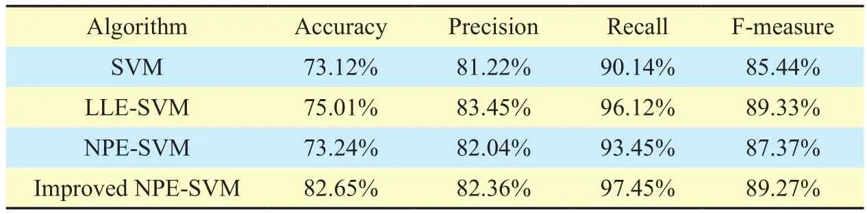
Table VI. Prediction result of data set PC5.
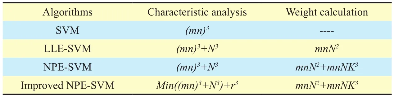
Table VII. Time Complexity of Algorithms.
ACKNOWLEDGEMENTS
This work is supported by the National Natural Science Foundation of China (Grant No.U1636115),the PAPD fund, the CICAEET fund, and the Open Foundation of Guizhou Provincial Key Laboratory of Public Big Data(2017BDKFJJ017).

Fig. 2. Comparison of the prediction results.
[1] Basili V R, Briand L C, Melo W L, “A Validation of ObjectOriented Design Metrics as Quality Indicators,” IEEE Transactions on Software Engineering,vol. 22,no. 10,1995,pp.751-761
[2] Emam K E, Benlarbi S, Goel N, et al, “Comparing case-based reasoning classifiers for predicting high risk software components,” Journal of Systems & Software,vol. 55, no. 3,2001,pp. 301-320.
[3] K.Ganesan,T.M.Khoshgoftar and E.B.Allen,” Casebased software quality prediction,” International Journal of Software Engineering & Knowledge Engineering, vol. 10,no. 2,2000,pp. 139-152.
[4] Khoshgoftaar T M, Allen E B, Jones W D, et al. “Classification-tree models of software-quality over multiple releases,” IEEE Transactions on Reliability, vol. 49,no. 1, 2000, pp. 4-11
[5] Khoshgoftaar T M, Seliya N. “Analogy-Based Practical Classification Rules for Software Quality Estimation”. Empirical Software Engineering,vol. 8, no. 4, 2003, pp. 325-350.
[6] Liao S, Ling X U, Yan M. “Software defect prediction using semi-supervised support vector machine with sampling”. Computer Engineering& Applications, 2017.
[7] Kokiopoulou E,Y Saad, “Orthogonal neighborhood preserving projections,” IEEE International Conference on Data Mining IEEE,vol. 29,2005,pp. 234-241.
[8] Zhang CS, Wang J, Zhao NY, Zhang D.”Reconstruction and analysis of multi—pose face images based on nonlinear dimensionality reduction,” Pattern Recognition,vol.37,no. 1,2004,pp.325-336.
[9] Bowes D, Hall T, Petrić J. “Software defect prediction: do different classifiers find the same defects “. Software Quality Journal,vol.1,2017,pp. 1-28.
[10] Yan Y,Guo P, “A Practice Guide of Software Aging Prediction in a Web Server Based on Machine Learning “, China Communications,vol.13,no. 6,2016,pp. 225-235
[11] Liqiang Zhang, Zhao, et al. “Dependence-Induced Risk: Security Metrics and Their Measurement Framework “.China Communications,vol.13,no. 11, 2016,pp. 119-128
[12] Zheng Z,Zibin J M, Tao G,et al. “Reliability prediction for internetware applications: a research framework and its practical use “. China Communications,vol. 12,no. 12,2015,pp. 13-20
[13] Zhang PH, et al. “A Novel Approach for QoS Prediction Based on Bayesian Combinational Model “. China Communications, vol. 13,no.11,2016,pp. 269-280
[14] Chengsheng Yuan, Xingming Sun, and Rui LV,“Fingerprint Liveness Detection Based on Multi-Scale LPQ and PCA,” China Communications,vol. 13, no. 7, 2016,pp. 60-65.
[15] Fu Y, Dong W, Yin L, et al.” Software Defect Prediction Model Based on the Combination of Machine Learning Algorithms “. Journal of Computer Research & Development, 2017.
[16] Malhotra R. “A systematic review of machine learning techniques for software fault prediction “. Applied Soft Computing Journal, vol.27,2015,pp. 504-518.
[17] Boehm B.” Industrial software metrics top 10 list“.IEEE Software,vol. 4,1987,pp.84-85
[18] Li M,Zhang H, Wu R, et a1.” Sample-based software defect prediction with active and semi-supervised learning “. Automated Software Engineering,vol. 19,no. 2,2012,pp. 201-230
[19] Roweis S T, Saul L K. “ Nonlinear Dimensionality Reduction by Locally Linear Embedding “. Science,vol. 290,no. 5500, 2000,pp. 2323-6.
[20] Zhang Z,Zha H. “ Principal Manifolds and Nonlinear Dimensionality Reduction via Tangent Space Alignment “. Society for Industrial and Applied Mathematics,2005.
[21] Wang Y,Wu Y. “ Complete neighborhood preserving embedding for face recognition “,Pattern Recognition,vol. 43,no. 3,2010,pp. 1008-1015
[22] Yajie Sun and Feihong Gu, “Compressive sensing of piezoelectric sensor response signal for phased array structural health monitoring,” International Journal of Sensor Networks, Vol. 23,No. 4,2017,pp. 258-264.
[23] Gu B, Sheng V S. “ A Robust Regularization Path Algorithm for ν-Support Vector Classification“.IEEE Transactions on Neural Networks & Learning Systems, vol. 28, no. 5, 2016, pp. 1241-1248.
[24] Bin Gu, Victor S. Sheng, Keng Yeow Tay,,Walter Romano,and Shuo Li,”Incremental Support Vector Learning for Ordinal Regression,” IEEE Transactions on Neural Networks and Learning Systems,vol. 26, no. 7, 2015,pp. 1403-1416.
[25] Challagulla V U B, Bastani F B, I-Ling Yen,Paul R A.” Em-pirical assessment of machine learning based software defect prediction techniques”,Proceedings of the 10th IEEE Interna-tional Workshop on Object-Oriented Real-Time Dependable Systems. Washington,DC,USA, 2005, pp. 263-270.
[26] Keerthi S S, Lin C J.” Asymptotic behaviors of support vector machines with Gaussian kernel “,Neural computation, 2003, pp. 1667-1668.
[27] Wang X H, Shu P, Cao L et al. “ A ROC curve method for performance evaluation of support vector machine with opti-mization strategy “.Computer Science Technology and Appli-cations,vol. 2, 2009, pp. 117-120.
杂志排行

China Communications的其它文章
- Geometric Mean Decomposition Based Hybrid Precoding for Millimeter-Wave Massive MIMO
- Outage Performance of Non-Orthogonal Multiple Access Based Unmanned Aerial Vehicles Satellite Networks
- Outage Probability Minimization for Low-Altitude UAV-Enabled Full-Duplex Mobile Relaying Systems
- Optimal Deployment Density for Maximum Coverage of Drone Small Cells
- Energy Efficient Multi-Antenna UAV-Enabled Mobile Relay
- Energy-Efficient Trajectory Planning for UAV-Aided Secure Communication