Optimal Deployment Density for Maximum Coverage of Drone Small Cells
2018-06-07ChaoDongJiejieXieHaipengDaiQihuiWuZhenQinZhiyongFeng
Chao Dong, Jiejie Xie,2,*, Haipeng Dai, Qihui Wu, Zhen Qin, Zhiyong Feng
1 The College of Communication Engineering, Army Engineering University of PLA, Nanjing 210007, China
2 The Unit 31106 of PLA, Nanjing 210007, China
3 The Department of Computer Science and Technology, Nanjing University, Nanjing 210093, China
4 The College of Electronic and Information Engineering, Nanjing University of Aeronautics and Astronautics, Nanjing 210016, China
5 Beijing University of Posts and Telecommunications, Beijing 100876, China
I. INTRODUCTION
Due to ease of deployment, low cost, high maneuverability, etc, Unmanned Areial Vehicles (UAVs) have been increasingly utilized in both military and civilian applications [1]-[4]. Among them, using Drone Small Cell(DSC) to provide communication service for ground users, i.e., mounting the wireless base station on a drone which is one kind of smallscale UAVs, has recently attracted significant attention [5]-[7]. The DSC can be deployed quickly to enable communication for scenarios under which the ground base stations are unavailable or crowded, e.g., earthquake, Center Business District (CBD) in the city, or soccer game, etc. Obviously, the coverage performance [8] is very important for the application popularization of DSC. Compared to single DSC, multiple DSCs can cooperate to provide a larger-scale communication service with higher flexibility, nevertheless, how to obtain maximum coverage performance for multiple DSCs is still a critical issue to be resolved.
Without loss of generality, a user is treated to be covered if its Signal to Interference plus Noise Ratio (SINR) is not lower than a threshold. Therefore, the coverage performance of DSCs can be in fluenced by many factors, such as altitude, transmission power, and deployment density, etc. Usually, the altitude and transmission power of DSCs are specified in advance, then the deployment density which is defined as the number of DSCs per unit area can be used to analyze that how many DSCs are needed to provide given coverage performance. Therefore, the deployment density of DSCs is important for the planner of DSC networks. In reality, when the deployment density of DSCs is too low, some users may be far from any DSC and cannot be covered with enough SINR due to the limited transmission power of the drones. On the contrary, with a high deployment density of DSCs, the small distance between DSCs would bring strong inter-cell interference, which can also decrease the SINR of some users and make them out of the coverage. To sum up, to achieve maximum coverage performance, an appropriate, rather than too low or too high, deployment density is desired.

Fig. 1. DSCs servering the ground users with LOS and NLOS links.
The coverage performance of DSCs has been well studied in recent years [4], [9]-[13].In [4], [9], and [10], the maximum coverage performance was studied without considering the inter-cell interference. In [12], the inter-cell interference between two DSCs was considered to study the coverage performance.In [13], the interference only from the nearest DSC was used to investigate the maximum coverage performance of multiple DSCs. Nevertheless, when multiple DSCs cooperatively provide the communication service to the ground users, the inter-cell interference occurs among all the DSCs, which is also known as cumulative inter-cell interference and should be considered. Therefore, current works cannot provide enough support to analyze the coverage performance with cumulative inter-cell interference among DSCs.
In this paper, we study the optimal deployment density of DSCs to achieve maximum coverage performance with cumulative inter-cell interference. First, we investigate the cumulative inter-cell interference of DSCs,where the challenge mainly comes from the air-to-ground channel model. As Figure 1 shows, although the DSCs have a great probability to use Line-of-Sight (LoS) links to communicate with ground users, the probability of Non-Line-of-Sight (NLoS) links cannot be neglected [9], [14]. Both links have different in fluence on the SINR of the ground users, and occurrence probabilities of both links are determined by the environment and the location of DSCs and users. Then, based on the cumulative inter-cell interference, we analyze the coverage performance of DSCs in term of altitude, deployment density, and coverage radius of single DSC, etc. Specifically, we build the optimal model to maximize the coverage performance in terms of the deployment density and the coverage radius of single DSC. Because there exists difficulty to obtain the optimal deployment density directly, we change the problem into finding the optimal coverage radius of single DSC to achieve maximum coverage performance. We prove that the coverage radius of single DSC has one-to-one relation with the deployment density, and propose an algorithm to compute it with low complexity.
Our main contributions are listed as follows.
(1) To the best of our knowledge, we for the first time study the optimal deployment density of DSCs for maximum coverage performance in the presence of cumulative inter-cell interference. We derive an approximate and closed-form expression of the cumulative inter-cell interference which comes from both probabilistic LoS and NLoS links.
(2) We analyze the coverage performance of DSCs and derive the transcendental function of optimal deployment density to obtain the maximum coverage. We propose an algorithm to get the near optimal result which only needs three iterations and has lower complexity compared to bisection algorithm.
(3) We execute field experiments with three 4-rotors drones and Matlab simulations to verify the correctness of the theoretical analysis.We also show some interesting phenomena on the relation between the deployment density and coverage performance through extensive numerical simulations. For example, increasing the transmission power of DSCs does not necessarily improve coverage performance,etc.
The rest of this paper is organized as follows. In Section II, we review related works.In Section III, we introduce models used in this paper and present the problem formulation. Then, we calculate the cumulative interference and solve the optimal deployment problem in Section IV. In Section V and VI,we present the evaluation results of the field experiments and the simulations. Finally, we conclude the paper in Section VII.
II. RELATED WORK
As we present in Section I, the cumulative inter-cell interference is the basis to analyze the coverage performance of DSCs. In this section, we introduce the related works regarding cumulative inter-cell interference firstly, and then present the state of art of the coverage performance for DSCs.
2.1 Cumulative inter-cell interference
For traditional terrestrial cellular networks,cumulative inter-cell interference is a fundamental element [15]. However, the air-toground channel is different from the groundto-ground channel, and hence the results from terrestrial cellular networks cannot be used in DSCs. There are many methods to model the interference in DSC networks and analyze the network performance [16], e.g., Poisson Point Process (PPP). For example, Zhang et.al in[17] modeled the DSC networks as a 3D PPP model, and calculated the cumulative interference imposed by all surrounding DSCs with the aid of the Laplace transform and the probability generating function [18]. Nevertheless,they only considered the LoS links, which is not realistic enough. Ravi et.al in [19] modeled a finite network of DSCs as a uniform Binomial Point Process (BPP) and derived exact expression for the coverage probability of a user located on the ground. However, whencalculating the cumulative inter-cell interference, they also did not put both probabilistic LoS and NLoS links into consideration.

Table I. List of notations.
2.2 Coverage performance of DSCs
There are many works investigating the coverage performance without considering interference [4], [9], [10]. For example, AI-Hourani et.al in [8] studied optimal deployment altitude of a drone providing maximum coverage and there is no inter-cell interference. However,when multiple drones work cooperatively, the inter-cell interference is not negligible. Mozaffari et.al in [20] investigated the coverage performance of a single DSC considering the interference from ground Device-to-Device(D2D) users, which is affected by the density of D2D users. A case where two DSCs interfere with each other was discussed in[13]. Mozaffari et.al studied the impact of inter-cell interference between two DSCs on the coverage performance, and showed that the inter-cell interference will significantly reduce coverage performance when the separation distance is small. Then, they found an optimal separation distance to achieve the maximum coverage. However, this work only considered two DSCs and cannot be extended to multiple DSCs easily. Mozaffari et.al in [12] investigated the maximum coverage performance of multiple DSCs in the presence of inter-cell interference. However, only the interference from the nearest DSC was considered. Lyu et.al in [21] sequentially placed the DSCs to provide wireless coverage for a group of users on the ground. However, they did not consider both LoS and NLos links when calculating the inter-cell interference.
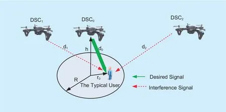
Fig. 2. Network model.
III. MODEL AND PROBLEM FORMULATION
In this section, we introduce the models used in this paper, including network model and air-to-ground channel model. After that, we present the problem formulation for maximizing the network coverage. Table 1 provides a summary of the major notations.
3.1 Network model
As shown in figure 2, consider a set K consisting of K DSCs deployed to provide communication service to ground users, and the DSCs are marked as DSC0to DSCK−1. As in[12], we assume that all DSCs locate at the same altitude represented by h. We define the coverage radius of each DSC as R, which is measured in the horizontal direction on the ground. As [16] does, we study the coverage performance of a typical user, and the results about the typical user can be converted to any user smoothly. We assume that the typical user is under the coverage of DSC0which is closest to the typical user. We must emphasize that because we use ideal path loss model in our study, the nearest DSC is basically equivalent to the one which leads to maximum received SINR. Then, we sort the DSCs by the diwhich is the crow- fly distance between the typical user and DSCi. We define rias the horizontal distance between a typical user and DSCi. Then, di=. As in [22], we assume that all DSCs follow a uniform random distribution, which is common for terrestrial base station distributions of practical cellular networks. We define the deployment density,i.e., the number of DSCs per square meter, as λ (Num/m2). Because that we only consider downlink communications, there are no interference from the other ground users, hereafter we call cumulative inter-cell interference as cumulative interference.
We assume that all the DSCs have the same transmit power Ptand share the same spectrum to provide the communication service to the ground users. Therefore, although the typical user is only served by its nearest DSC,i.e., DSC0, it would suffer the cumulative interference from the other DSCs. Obviously,the coverage performance can be influenced seriously by the cumulative interference which is related to characters of the air-to-ground channel. Next, we introduce the air-to-ground channel model used in this paper.
3.2 Air-to-ground channel model
Due to the non-ignorable probability for both of LoS and NLOS connectivity, the air-toground channel of DSCs is different from the traditional terrestrial channel. As discussed in[9] and [14], there are two main propagation links including LoS links and NLoS links between the DSCs and the ground users. And each kind of link has a specific probability of occurrence which depends on the environment, the altitude of DSCs h and the horizontal distance ri, etc. In this paper, we consider both LoS and NLoS links to model the channel from DSCs to the ground users. Therefore,the received signal power Pr( ri) of the typical user from DSCiis
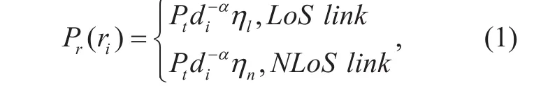
where α is the path loss exponent which mainly depends on the distance to represent the large-scale fading effect and α> 2, ηland ηnare additional attenuation factors corresponding to the small-scale fading effect of LoS and NLoS links, respectively. Note that ηnis smaller than ηldue to the shadow effect on NLoS links.
From [9] and [14], LoS and NLoS links have different probabilities of occurrence separately. Among them, the probability of LoS link from DSCito the typical user, i.e.,Prl(ri), is given by [8]

where a and b are constant values which depend on surrounding environment (suburban,urban, dense urban, high-rise urban and so on), and. Naturally, the NLoS probability, which is the probability of NLoS link between DSCiand the typical user is

Therefore, the average received signal power of the typical user from DSCiis

Let, then the average received signal power can be rewritten as

As mentioned before, we assume that the typical user is under the coverage of DSC0.Then,, and the SINR at the typical user is given by

where N is the noise, and I is the cumulative interference from other DSCs, which is

3.3 Problem formulation
In this paper, we intend to find the optimal deployment density to achieve maximum coverage performance with both LOS and NLoS Links. To facilitate analysis, the coverage performance is measured by coverage ratio,which is the ratio of covered area to the overall network area which refers to the size of a predefined area covering all the ground users.
To investigate this problem, we define that a user is covered by DSCs if the SINR at its position is greater than a threshold ε which is not less than 0 dB in this paper. Then the average effective coverage area of a DSC is cR2, where c is an empirically chosen factor called area factor in this paper. For example, if the average effective coverage area of a DSC is calculated as a hexagonal one, we have c=3/2, and c would be π when the average effective coverage area is calculated as a circular with a radius of R. As ε is not less than 0 dB and all DSCs share an underlay spectrum, there is no overlap between the coverage areas. Because that the DSCs follow a uniform random distribution, thus the overall effective coverage areas is given as KcR2.Then, the deployment density of DSCs λ (the number of DSCs per square meter, Num/m2),can be defined asand the coverage ratio is given by

In addition, as R is the coverage radius of a DSC, the user located at the coverage edge can still meet the SINR requirement. Therefore, the optimization problem can be written as

IV. THEORETICAL ANALYSIS
To accurately analyze the coverage performance of DSCs and determine the optimal deployment density, the SINRs of the users are needed to be analyzed, especially for the users locating at the coverage edge of their nearest DSCs. In this section, we would calculate the cumulative interference and derive an approximate and closed-form expression for it. After that, we analyze the coverage performance of DSCs and propose a low complexity algorithm to determine the optimal deployment density that achieves the maximum coverage ratio.
4.1 Cumulative inter-cell interference
As mentioned before, to calculate the cumulative interference at a typical user, the characters of the air-to-ground channel must be considered. Due to the different probabilities of LOS and NLoS links, the Laplace transform and probability generating function in commonly used Poisson model will bring huge computational complexity. To overcome this,we model the interference through Equivalent Uniform Density Plane-Entity (EUDPE) method [22], which can be used to calculate the cumulative inter-cell interference to analyze the coverage performance for all the existing BS distribution models and has similar results compared with Poisson model. Because that all DSCs follow a uniform random distribution and a large-scale DSC networks are considered in this paper, we can model the DSCs as an equivalent uniform density plane entity and calculate the cumulative interference through EUDPE method. As the horizontal distance between the typical user and the nearest interference DSC should not be less than R, the cumulative interference at typical user is given by

where Δriis the distance difference in horizontal direction from the typical user to DSCiand DSCi+1, i.e., Δri=ri+1−ri. In addition, dˆ and rˆ are temporary variables and will not appear in the final results. Here, step (a) follows the EUDPE method. As α> 0,→0 when the distance diis large enough. Meanwhile,when i is large enough, meaning that the interference from the DSC far away is very small. Accordingly, step (b) comes from the assumption that a large-scale DSC networks is considered and the upper limit of integration is in finity.
Next, to facilitate the computation of optimal deployment density, we derive an approximate and closed-form expression for the cumulative interference.
Theorem 1:The approximate and closedform expression for the cumulative interference is given by

where k ranges fromto 1, and dR=.
Proof:We ignore the constant component in Formula (11), and becausethen

Therefore,

where in the derivation process,

Note that step (a) in Formula (13) follows the utilization of integration by parts,and the next two steps come from slight enlargement. From above derivation, we can know thatis larger thanwhile smaller than. Thus, the expression of the cumulative interference can be approximated as, where k is a parameter andAt this point, we obtain the approximate and closed form expressions of the cumulative interference.
In this paper, we set k to 0.9 because the lower bound of k is about 0.9. We compare the cumulative interference calculated by Theorem 1 (approximate) with the non-approximate one in Figure 3. As shown, the results obtained by Theorem 1 coincide with the non-approximate one, which verifies the correctness and accuracy of Theorem 1. Next,we investigate the optimal deployment density to achieve the maximum coverage based on this Theorem.
4.2 Optimal deployment density
From Formula (8), the coverage ratio is influenced by both the coverage radius R and deployment density λ. In fact, R and λ will interact with each other. Hence, to get the optimal deployment density for achieving maximum coverage performance, it is necessary to study the relation between R and λ.

Fig. 3. Cumulative interference power vs. R when k=0.9.
Remark 1:The relation between the deployment density and coverage radius can be represented as

Proof:We consider the coverage performance at the typical user which locates at the coverage edge of nearest DSC. It is reasonable to assume the SINR at this user is equal to ε.We letand substitute Formula (5)and (11) into this equation,

And the equation can be rewritten as

Remark 2:The coverage radius decreases monotonically with the deployment density,and there is a one-to-one relationship between them.
Proof:Derived from Formula (15), we can know, which means that R decreases monotonically with λ, and there is a one-toone relationship between R and λ. The detailed proof can be found in APPENDIX A.
Now we intend to find the optimal deployment density. However, as it is difficult to derive the explicit expressions of Ratio in terms of λ, we cannot obtain the optimal density directly. Based on Remark 1 and 2, we can solve the optimization problem by determining the coverage radius corresponding to the optimal deployment density, and then obtain the latter.

Algorithm 1. The algorithm for calculating Ropt.Input: P h N b c Accuracy α ε η η Output: R R t ,,,,,,,, ,l n s, b 1: Initialize Rs=0+, Rb=∞2: While R-R > Accuracy b s do 3: f = f(R)v b, g = g(R)v a s 4: Rs← the positive real root of W( R, f,g) 0 v v=5: f = f(R)v s, g = g(R)v a b 6: Rb← the positive real root of W( R, f,g) 0 v v =7: end while 8: return R R s, b
By substituting Formula (15), the Formula(8) can be rewritten as

Now, the coverage ratio is expressed as a function of R. To find the trend of coverage ratio, we take the derivative of this objective function, and obtain that

where f'(R) and ga(R) are given in Section(IV-A). And we make

It is easy to prove thatis always greater than 0, thus the extreme point would be determined by W( R) = 0.Noting that,is the average received signal power, which decreases as R increases. When R is a smaller value, the value ofis very large while the value ofis small, thus W( R) is greater than 0. And when R is a larger value, the opposite is true,i.e., W( R)<0. Therefore, there is an extreme point where the maximum coverage ratio can be obtained, and the extreme point Roptis the root of W( R)=0.
By Remark 2, the coverage ratio increases as λ increases up to the optimal point λopt, and after that it will decrease. Once Roptis determined, λoptcan be obtained by λopt=Y( Ropt). But it’s difficult to determine λoptdirectly. Next, we propose an algorithm with low complexity to determine Ropt, and thereby, obtain the optimal deployment density λopt.
As W( R) is a transcendental function, it is difficult to get the solution of W( R)=0 in closed form. Thus, we solve the function by numerical method. We propose an algorithm to determine Roptby changing the problem of finding out the root of the transcendental function into the one of solving multiple polynomial functions.
In W( R), the existence of f( R) and ga(R) increases the computational complexity of W( R)=0. If the values of f( R)and ga(R) are determined, W( R)=0 could be transformed into a polynomial function.Therefore, based on Formula (18), we make

where fvand gvare temporary variables. Note that, when fv> f( Ropt) and gv< ga(Ropt), the positive real root of W( R, fv,gv) = 0 is slightly larger than Ropt, while the positive real root of W( R, fv,gv) = 0 is slightly smaller than Roptwhen fv< f( Ropt) and gv> ga(Ropt). As f( R) and ga(R) decrease slightly with increasing R, we can assign values to fvand gvin each iteration to gradually approach f( Ropt)and ga(Ropt), and finally obtain approximations of Ropt. The specific algorithm is shown in Algorithm 1. Rsand Rbare approximations of λopt. Hence, the approximations of the optimal deployment density can be obtained as λopt−b=Y( Rs) and λopt−s=Y( Rb).
Note that, Algorithm 1 needs multiple iterations to get the optimal result. In each iteration, we solve W( R, fv,gv) = 0 in polynomial time by generating the companion matrix and calculating the eigenvector of this matrix.We compare the convergence performance between Algorithm 1 and the bisection algorithm which is usually used to solve nonlinear equation. As shown in Figure 4, our proposed algorithm can converge more quickly than the bisection algorithm. Note that, only three iterations is needed to get sufficiently accurate approximations of Ropt, then the near-optimal solution of λoptwith an accuracy of about 10−2can be obtained.
V. VALIDITY
In this section, we verify the correctness of the theoretical analysis through field experiment and Matlab simulation. Due to the limitation of the experiment conditions, e.g., the maximum transmit power of the radio module on the drone, we adopt different parameters for experiment and simulation. The field experiment is used for small-scale DSC networks and the Matlab simulations is for large-scale DSC networks.

Fig. 4. Convergence performance.

Fig. 5. Field experiment.
5.1 Field experiment
In this subsection, we verify the relation trend between the coverage ratio and deployment density through comparing the experiment results with numerical calculation.
5.1.1 Experiment setting
As shown in figure 5, we use three 4-rotors drones to act as DSCs in the air and one USRP N210 for a typical user on the ground.The drone we use is a 4-rotors one which can hover at an altitude of about 10 m. On each drone we use a Raspberry Pi to control a radio module (HackRF One) to provide communication service on 2.4 GHz with the transmission power of 10 dBm at most. To ensure fairness,we adopt the same parameters in numerical calculation, i.e., the altitude, the frequency,and DSC transmit power.
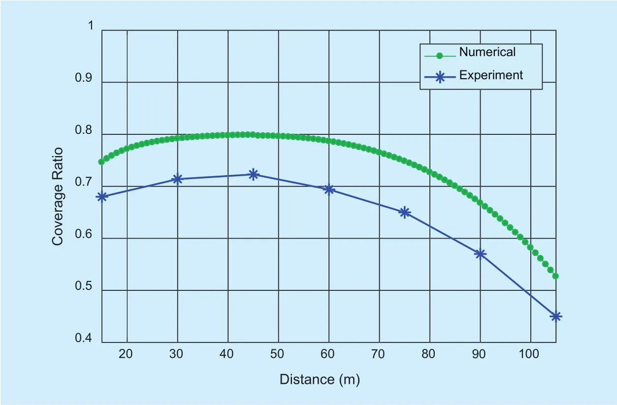
Fig. 6. Field experiment results.
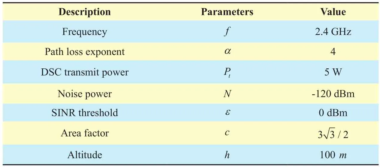
Table II. Simulation parameters.
5.1.2 Experiment results
We change the distance between three drones to represent different deployment density.Then through moving the ground user to different locations, we obtain the coverage ratio.For each set of parameter choice and location,we run the experiments 50 times and compute the average value. The results can be found in optimal deployment density to achieve the maximum coverage ratio, and the variation trends of both lines are almost identical.when the distance is bigger, the coverage ratio increases as the distance decreases. On the contrary, when the distance is smaller, i.e., λ is bigger, the coverage ratio will decrease with the decrease of the distance. In addition, we notice that due to the environment uncontrollability in reality, for example, the path loss and noise power, the coverage ratio of field experiments is not that smooth and less than the one obtained through numerical simulations.
5.2 Simulation
In this subsection, we compare the results of Matlab simulation and numerical calculation.
5.2.1 Simulation setting
To ensure the reasonableness of the results,we adopt the same parameters listed in table 2 for simulation and corresponding numerical calculation. In this comparison, we use a number of DSCs to cover a 100 km×100 km field, then the number of DSCs can be calculated by 1010×λ. We assume that these DSCs follow a uniform random distribution, and the ground users follow Poisson Point Procedure(PPP). For each set of parameter choices, we run the simulations 500 times and average the obtained values.
5.2.2 Simulation results
From figure 7, for both lines, we can see that when λ<λopt, the coverage ratio increases as λ becomes bigger. On the contrary, when λ>λopt, the coverage ratio will decrease with the increase of λ. Meanwhile, the trend of coverage ratio obtained in simulations is consistent with the one of numerical simulation. Based on numerical calculation, we have λopt=3.41× 10⁻⁷. For simulations, the achieved λoptis almost the same. Meanwhile, λ=3.41× 10⁻⁷indicates that there are 3410 DSCs in the simulation region which is 100 km×100 km . We notice that the coverage ratio of simulation is slightly less than the one calculated by theoretical analysis. The reason is as follows: due to the randomness in Matlab simulation, the placement of DSCs is not as uniform as in numerical calculation. Some DSCs may be distributed relatively dense and they will have more overlapping coverage area. Therefore, the whole coverage area will shrink and the coverage ratio of Matlab simulation is slightly less than the one calculated by theoretical analysis.
VI. PERFORMANCE EVALUATION
In this section, to further study the coverage performance of DSC networks, we study the influence of different factors, i.e., altitude,transmission power, and environment, on the relation between the coverage ratio and optimal deployment density. Following [9], [14],[23], we set four different types of environment through changing the values of a, b,ηl, and ηnas shown in table 3. If not specified, the parameters used in the evaluation are following table 2 and the default environment is Urban.
6.1 Altitude
We select three altitudes in this evaluation,i.e., 100 m, 200 m and 300 m. From figure 8a, we can see that for a given altitude, there indeed exists an optimal deployment density,i.e., λopt, to achieve the maximum coverage ratio. It is worthwhile to note that a higheraltitude brings a slightly bigger coverage ratio when λ<λopt, while the opposite thing happens when λ>λopt. We analyze the reason through studying the coverage radius of a single DSC. Increasing the altitude leads to an increase in the crow- fly distance between the users and DSCs, which results in an increase in path loss, a decrease in the received signal power and the interference power. Meanwhile,increasing the altitude may also bring the increase in the probability of LoS link which will increase the received signal power. When DSCs are deployed at higher density, users would suffer serious cumulative interference from nearby DSCs. Therefore, the coverage radius of single DSC is smaller, and the angle of evaluation between a single DSC and its coverage area border is bigger. That is to say,the probability of LoS link for single DSC coverage is bigger when λ is higher. Under this condition, when the altitude increases, the increase of the path loss is more obvious than the increase in the probability of LoS link, this will result in a decrease in SINR and then a reduction in the coverage radius. While, when deployed at lower density, the interference is low and the DSC networks become a noise limited network rather than an interference limited one, in which the coverage radius is mainly determined by the desired signal and noise power. Then higher altitude brings higher probability for LoS links, which results in a stronger desired signal and a greater coverage radius as shown in figure 8b. Finally, the coverage ratio changes with the coverage radius accordingly. In addition, we notice that for a given altitude, the coverage radius decreases with the increase of deployment density. The reason is as follows: for a typical user, the received signal strength does not change due to the fixed distance from the DSC. However, the cumulative interference brought by the DSCs nearby increases. Then the SINR decreases and the coverage radius of single DSC will decrease.

Table III. Environment parameters.

Fig. 7. Comparison of simulation and numerical calculation.
6.2 Transmission power

Fig. 8. Coverage performance versus altitude.

Fig. 9. Coverage performance versus transmission power.
Figure 9. shows the impact of transmission power on the coverage performance. We can see that there still exists an optimal deployment density for a given transmission power from figure 9a. A bigger transmission power represents a bigger coverage ratio when λ<λopt, while the phenomena is no longer obvious as λ>λopt. As we know, the powers of desired signal and cumulative interference both increase with the transmission power.When DSCs are deployed at high density, users suffer from serious interference, and the DCS network is an interference limited one.That is to say, although the desired power and cumulative interference power increase at the same time, the latter is more. Therefore, increasing transmission power cannot improve coverage performance when the deployment density is high. On the contrary, when DSCs are deployed at low density, the DSC network is a noise limited one. Increasing transmission power leads to an increase in desired signal strength, leading to an improvement in coverage performance. Therefore, increasing the transmission power of DSCs does not necessarily improve coverage performance. Besides,we can see that the coverage radius increases as the deployment density decreases from figure 9b. This is because for a given transmission power, the decrease of deployment density represents less cumulative interference.
6.3 Environment
We consider four different types of environment listed in table 3 in this evaluation. As shown in figure 10, we can observe that the DSC networks deployed at suburban has the best coverage performance, and the worst happens for the high-rise urban. The reason is that the LOS links is dominant for suburban while the probability of NLoS links is more higher for high-rise urban. We also notice that the coverage performances in different environments are similar when the deployment density is high. This is because that the coverage performance is limited by serious cumulative interference, and when DSCs are deployed at same high density, the cumulative interference powers for different environments are similar.
Figure 11. shows the optimal deployment density of DSCs at different altitudes in different environments.
We can observe that the optimal deployment density goes down with the altitude of DSCs for all environments. As the increase in altitude leads to increased cumulative interference, DSCs need to be deployed sparsely to reduce the impact of interference. As a result, lower optimal deployment density is obtained when the altitude of DSCs increases.But we must note that if the altitude increases furtherly, the coverage area of single DSC may decrease, thus the optimal deployment density may go up. Accordingly, from Figure 12 we can see that the maximum coverage ratio obtained when DSCs are deployed at optimal density decreases correspondingly as the altitude increases for all environments. And we can observe that the best coverage performance can be always achieved for suburban when the DSCs are deployed with optimal deployment density.
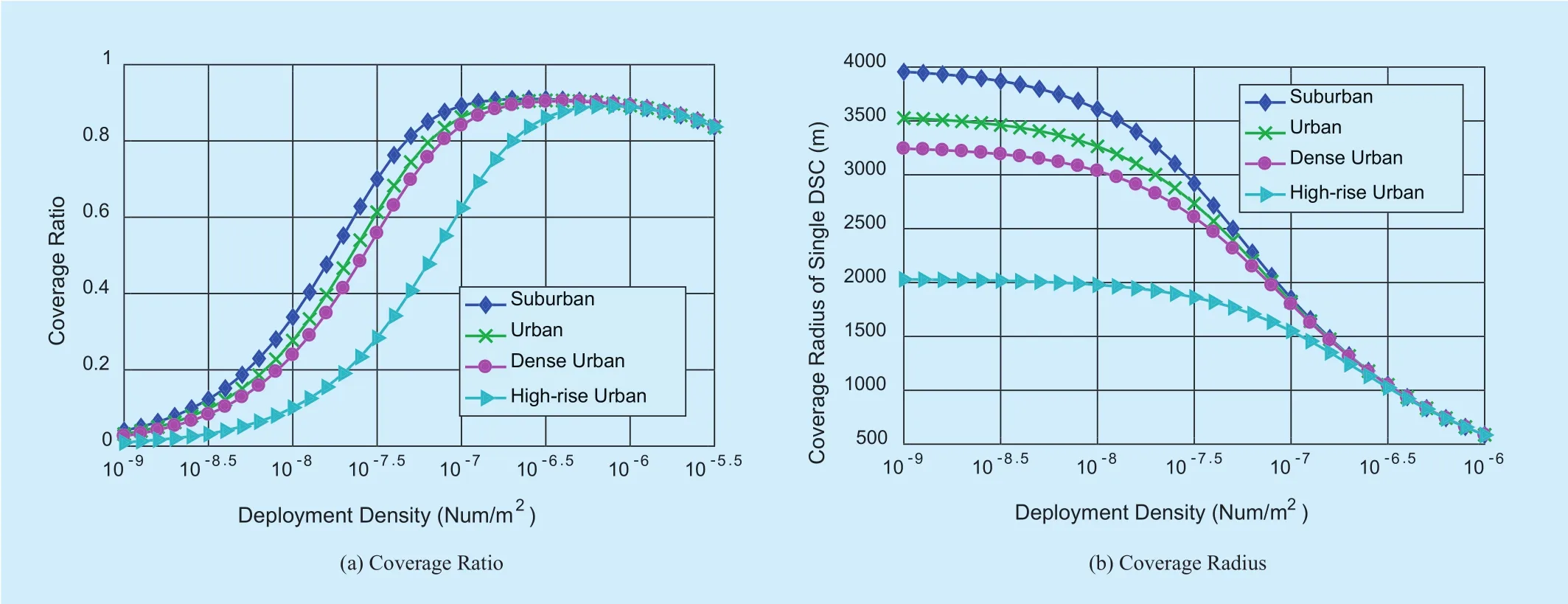
Fig. 10. Coverage Performance versus Environment.
VII. CONCLUSION

Fig. 11. Optimal deployment density versus altitude in different environments.

Fig. 12. Maximum coverage ratio versus altitude in different environments.
In this paper, we investigate the coverage performance of multiple DSCs in consideration of cumulative inter-cell interference. Especially,we consider both probabilistic LoS and NLoS links to model the air-to-ground channel of DSC networks. To get the optimal deployment density, we calculate the cumulative inter-cell interference using the EUDPE method firstly,and then determine the extreme point which achieves maximum coverage ratio and propose an algorithm to calculate the optimal deployment density. We verify the correctness of the theoretical analysis through field experiments and Matlab simulations. From our evaluation results, we found some interesting phenomena such as increasing the transmission power of DSCs does not necessarily improve coverage performance. In the near future, we will study how to deploy the DSC networks with maximum coverage in reality.
ACKNOWLEDGEMENTS
This work is supported in part by National NSF of China under Grant No.61472445, No.61631020, No. 61702525 and No. 61702545,in part by the NSF of Jiangsu Province under Grant No. BK20140076.5.
APPENDIX A PROOF OF THEMONOTONICITY OF R
Take the derivative of Formula (14), we have

where f′(R) and g Ra() are given in Section(IV-A). Step (a) comes from the substitution of Formula (14). From the above derivation, we can know<0. Therefore, we can obtain that
indicating that R decreases monotonically with λ, and there is a one-to-one relationship between them.
[1] I. Bekmezci, O. K. Sahingoz, and S. Temel, “Flying ad-hoc networks(fanets): A survey,” Ad Hoc Networks, vol. 11, no. 3, pp. 1254-1270, May 2013.
[2] C. Barrado, R. Messeguer, J. Lopez, E. Pastor, E.Santamaria, and P. Royo, “Wildfire monitoring using a mixed air-ground mobile network,” IEEE Pervasive Computing, vol. 9, no. 4, pp. 24-32,Dec. 2010.
[3] J. George, S. P. B, and J. B. Sousa, “Search strategies for multiple uav search and destroy missions,” Journal of Intelligent Robotic Systems, vol.61, no. 4, pp. 355-367, Jan. 2011.
[4] M. Alzenad, A. El-keyi, F. Lagum, and H. Yanikomeroglu, “3d placement of an unmanned aerial vehicle base station for maximum coverage of users with different qos requirements,” IEEE Wireless Communications Letters, vol. PP, no. 99,pp. 1–1, Sep. 2017.
[5] S. Hayat, E. Yanmaz, and R. Muzaffar, “Survey on unmanned aerial vehicle networks for civil applications: A communications viewpoint,” IEEE Communications Surveys Tutorials, vol. 18, no.4, pp. 2624–2661, Apr. 2016.
[6] S. Chandrasekharan, K. Gomez, A. Al-Hourani, S.Kandeepan, T. Rasheed, L. Goratti, L. Reynaud,D. Grace, I. Bucaille, T. Wirth, and S. Allsopp,“Designing and implementing future aerial communication networks,” IEEE Communications Magazine, vol. 54, no. 5, pp. 26–34, May 2016.
[7] Y. Zeng, R. Zhang, and T. J. Lim, “Wireless communications with unmanned aerial vehicles:opportunities and challenges,” IEEE Communications Magazine. vol. 54, no. 5, pp. 36-42, May 2016.
[8] K. Daniel, S. Rohde, and C. Wietfeld, “Leveraging public wireless communication infrastructures for uav-based sensor networks,” in Proc. IEEE International Conference on Technologies for Homeland Security(HST), Nov. 2010, pp. 179-184.
[9] A. Al-Hourani, S. Kandeepan, and S. Lardner,“Optimal lap altitude for maximum coverage,”IEEE Wireless Communications Letters, vol. 3, no.6, pp. 569–572, Jul. 2014.
[10] R. I. Bor-Yaliniz, A. El-Keyi, and H. Yanikomeroglu, “Efficient 3-d placement of an aerial base station in next generation cellular networks,” in Proc. IEEE International Conference on Communications (ICC), May 2016, pp. 179-184.
[11] M. M. Azari, F. Rosas, K. C. Chen, and S. Pollin,“Optimal uav positioning for terrestrial-aerial communication in presence of fading,” in Proc.IEEE Global Communications Conference (GLOBECOM), Dec. 2016, pp. 1-7.
[12] M. Mozaffari, W. Saad, M. Bennis, and M.Debbah, “Efficient deployment of multiple unmanned aerial vehicles for optimal wireless coverage,” IEEE Communications Letters, vol. 20,no. 8, pp. 1647–1650, Aug. 2016.
[13] M. Mozaffari, W. Saad, M. Bennis, and M. Debbah, “Drone small cells in the clouds: Design,deployment and performance analysis,” in Proc.IEEE Global Communications Conference (GLOBECOM), Dec. 2015, pp. 1-6.
[14] A. Al-Hourani, S. Kandeepan, and A. Jamalipour,“Modeling air to ground path loss for low altitude platforms in urban environments,” in Proc.IEEE Global Communications Conference (GLOBECOM), Dec. 2014, pp. 2898 - 2904.
[15] N. H. Mahmood, K. I. Pedersen, and P. Mogensen, “Interference aware inter-cell rank coordination for 5g systems,” IEEE Access, vol. 5,pp. 2339–2350, Feb. 2017.
[16] H. ElSawy, A. Sultan-Salem, M. S. Alouini, and M. Z. Win, “Modeling and analysis of cellular networks using stochastic geometry: A tutorial,”IEEE Communications Surveys Tutorials, vol. 19,no. 1, pp. 167–203, Nov. 2017.
[17] C. Zhang and W. Zhang, “Spectrum sharing for drone networks,” IEEE Journal on Selected Areas in Communications, vol. 35, no. 1, pp. 136–144,Jan. 2017.
[18] J. G. Andrews, F. Baccelli, and R. K. Ganti, “A tractable approach to coverage and rate in cellular networks,” IEEE Transactions on Communications, vol. 59, no. 11, pp. 3122–3134, Oct. 2011.
[19] V. V. C. Ravi and H. S. Dhillon, “Downlink coverage probability in a finite network of unmanned aerial vehicle (uav) base stations,” in Proc. IEEE 17th International Workshop on Signal Processing Advances in Wireless Communications(SPAWC), Aug. 2016, pp. 1-5.
[20] M. Mozaffari, W. Saad, M. Bennis, and M. Debbah, “Unmanned aerial vehicle with underlaid device-to-device communications: Performance and tradeoffs,” IEEE Transactions on Wireless Communications, vol. 15, no. 6, pp. 3949–3963,Feb. 2016.
[21] J. Lyu, Y. Zeng, R. Zhang, and T. J. Lim, “Placement Optimization of UAV-Mounted Mobile Base Stations”, IEEE Communication Letters, vol. 21,no. 3, pp. 604-607, Mar. 2017.
[22] H. Zhang, S. Chen, L. Feng, Y. Xie, and L. Hanzo,“A universal approach to coverage probability and throughput analysis for cellular networks,”IEEE Transactions on Vehicular Technology, vol.64, no. 9, pp. 4245–4256, Sep. 2015.
[23] R. I. Bor-Yaliniz, A. El-Keyi, and H. Yanikomeroglu, “Efficient 3-d placement of an aerial base station in next generation cellular networks,” in Proc. IEEE International Communications Conference (ICC), May 2016, pp. 1-5.
杂志排行

China Communications的其它文章
- Geometric Mean Decomposition Based Hybrid Precoding for Millimeter-Wave Massive MIMO
- Outage Performance of Non-Orthogonal Multiple Access Based Unmanned Aerial Vehicles Satellite Networks
- Outage Probability Minimization for Low-Altitude UAV-Enabled Full-Duplex Mobile Relaying Systems
- Energy Efficient Multi-Antenna UAV-Enabled Mobile Relay
- Energy-Efficient Trajectory Planning for UAV-Aided Secure Communication
- An Enhanced Direct Anonymous Attestation Scheme with Mutual Authentication for Network-Connected UAV Communication Systems