Adaptive slices for acquisition of anisotropic BRDF

Radomr Vvra,Ji Filip()

The Author(s)2017.This article is published with open access at Springerlink.com

1 Introduction

Realistic appearance of spatially homogeneous materialsisusually represented by means of a bidirectional reflectance distribution function(BRDF) as introduced in Ref. [1]. Precise measurement of the BRDF is time consuming due to the very high number of samples of the function that have to be taken.In this paper,we introduce a method for adaptive measurement of the BRDF that provides precise results even when using a limited number of samples.The method does not rely on a database of already measured materials and scales well,so it is applicable where precision is important.We build upon the method in Ref.[2]which measures the BRDF by one-dimensional slices,but substantially extend its contributions.

We note that the BRDF is a four-dimensional vector-valued functionfr(θi,θv,ϕi,ϕv) of the illumination directionωi=[θi,ϕi]and the viewing directionωv=[θv,ϕv];itdefines how lightis reflected from a material(see Fig.1).The isotropic BRDF is a three-dimensional simplification of the BRDF which can represent only a subclass of spatially homogeneous materials such as plastics or paints.In contrast,the full-dimensional BRDF is anisotropic.Anisotropic materials have variable reflectance when rotated around a surface normal,as commonly found for many real-world materials that contain directional elements such as fabric threads or wood grain.

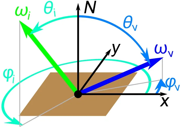
Fig.1 Parameterization of the BRDF.

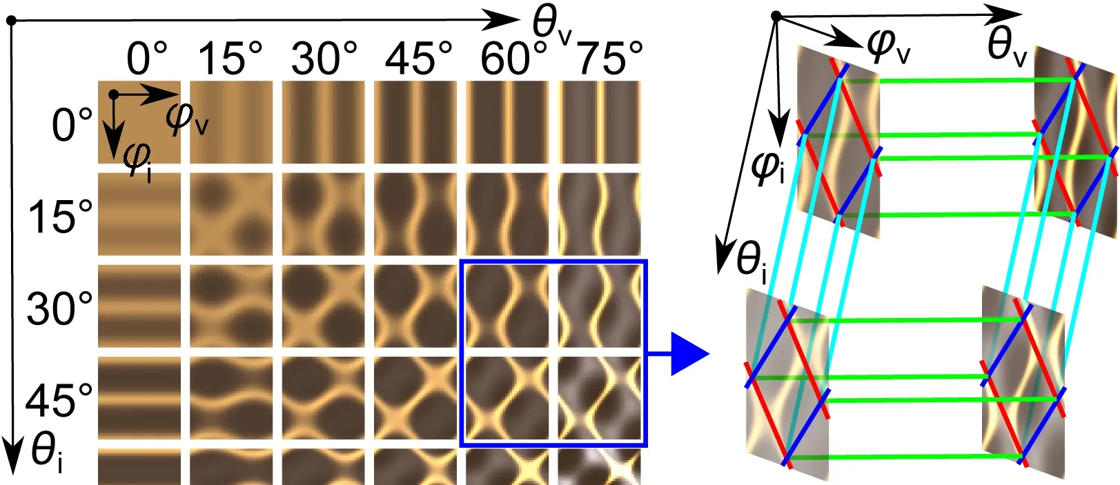
Fig.2 Visualization of a BRDF with highlighted axial(red),diagonal(blue),horizontal(green),and vertical(cyan)slices.Note that the BRDF is a four-dimensional continuous function and that its axes are orthogonal.

The proposed method is based on our findings concerning the typical behavior of anisotropic BRDFs. We assume that each two-dimensional BRDF subspace with fixedθi,θv(see Fig.2)and its important features can be captured by several diagonal and anti-diagonal cross-sections(so-calledslices),i.e.,one-dimensional signals.Sampling the BRDF subspace only along the slices greatly reduces the number of samples needed(see Ref.[2]).Another saving is made by choosing only certain subspaces(e.g.,by limiting values ofθi,θvto multiples of 15°:see Fig.2(left)).Subsequently,elevation-dependent behavior is captured by another type of slice:see Fig.2(right).The slices form a sparse 4D structure in BRDF space.Their ability to capture important features of the BRDF depends on their density.The more dense the sampling,the more precise reconstruction that can be achieved,but at the cost of more samples.In order to balance measurement time and reconstruction quality,we thus provide optimal con figurations of such a sampling structure with respect to a chosen number of samples.

Although the structure itself substantially reduces the number of BRDF samples in comparison to dense regular sampling,we must reduce further the number of measured values to make the method practical.This is done by using sparse,adaptive sampling along individual slices.

Although there are approaches to efficient material appearance measurement using specific lighting systems,using,e.g.,basis-illumination[3]or linear light sources [4], we focus on a sequential measurement process as typically used by goniometric devices having a single point-light source and a single accurate sensing device.

The main contribution of this paper is,to the best of our knowledge,the first adaptive method for precise measurement of the full 4D anisotropic BRDF which does not rely on a database of already measured materials.

Section 2 outlines our research in the context of related work,while Section 3 explains the principle of the BRDF slices.Section 4 proposes a heuristic algorithm for adaptive measurement of values along them.Missing data reconstruction from the slices is explained in Section 5 and optimal placement of the slices in BRDF space is analyzed in Section 6. Section 7 compares the proposed method with two interpolation methods that work with nearly-uniformly distributed samples,using simulated-and real-measurement scenarios. We also compare our method with a previous adaptive method[2].Finally,Section 8 discusses advantages and limitationsof themethod and Section 9 concludes the paper.

2 Related work

The main objective of this paper is an approach for adaptive acquisition of the BRDF that uses a limited set of samples.Our methods of adaptive measurement and data interpolation are closely related,as our task is to reconstruct an unknown function well by optimal placement of novel on previously measured values.This optimal placement depends on the chosen interpolation method.Good candidates are global interpolation methods[5]based on radial basis functions(RBF)or kriging.Although these methods might seem suited to solving the problem of adaptive sampling for measurement of material appearance,they have high computational demands which become intractable when the number of samples exceeds several thousands.Adaptive measurement of material appearance is investigated in Ref.[6],but only in two dimensions;the approach samples the reflectance field.An adaptive approach for image-based BRDF measurement is proposed in Ref.[7],with planning of viewing and illumination directions based on minimization of uncertainty in parameters of an analytical model.Nauyoks et al.[8]fi t six isotropic BRDF models to the measured data.They iteratively add new samples by including illumination and viewing directions where the models predict different outputs,i.e.,the models disagree.Some goniometers[9]use a two pass adaptive method, first making a full pass over the outgoing hemisphere,and then making a fine pass around the detected specular peak in the form of a spiral pattern.

Matusik et al.[10]represent isotropic BRDFs using a wavelet basis or a linear combination of BRDFs.Similarly,Nll et al.[11]represent the same BRDFs using basis functions;however,deviations of their reconstruction from the reference are approximated by a basis of correction functions.Nielsen et al.[12]present an approach to reconstructing isotropic BRDFs from basis functions using extremely sparse measurements,while Vavra and Filip[13]have extended their approach to anisotropic BRDFs.These approaches optimize a set of appropriate directional samples based on information in a database;however,they are not adaptive(except for Ref.[13])according to the measured materials.As a result,they cannot precisely measure materials with features not present in the database.

None of the methods above provide a reliable way to effectively acquire dense BRDF data without knowledge of previously recorded BRDFs.On the other hand,several interpolation methods applicable to measured samples exist,based on,for instance,barycentric interpolation[14],thin plate splines[15],oraGaussian pyramid in theso-called pull–push algorithm[16]. Recently,Ward et al.[9]reconstruct uniformly sampled BRDF measurements by interpolated radial basis functions using a mass transport solution.

Another option is displacement interpolation[17]based on solving the generalized mass transport optimization problem. It performs well,but its computational demands increase dramatically when the number of samples is in the order of thousands,and therefore factorization is required.An alternative approach to BRDF data interpolation is to use data factorization by Tucker decomposition[18].This can represent both isotropic and anisotropic BRDFs with quality comparable to analytic BRDF models in reasonable reconstruction time.

As these interpolation methods differ in quality and speed,we have tested several of them and selected two as references for evaluation of our proposed approach based on adaptive measurement.

Our paper builds on Ref.[2]which uses slices to capture the main features of 2D subspaces of the BRDF.Values on the slices are measured adaptively to minimize the number required.Although individual subspaces can be captured very precisely,the whole BRDF is obtained by simple interpolation and is therefore rather inaccurate.In this paper,we introduce two new types of slices that enable us to capture all important features and to achieve better BRDF reconstruction quality.The adaptive sampling algorithm is enhanced to enable very efficient sampling of the slices based on a chosen count of samples.This allows control over the time needed by the measurement process,which is very important in industrial practice.We also consider the optimal placement of the slices,which is very important for achieving good results.This topic is completely overlooked in Ref.[2].

3 One-dimensional BRDF slices

3.1 Introduction

The BRDF is a four-dimensional vector-valued function of the elevation anglesθi,θvand the azimuthal anglesϕi,ϕv.To enable efficient sampling of the entire BRDF,we propose to use four types of one-dimensionalslices. Two types,axialanddiagonalslices,were introduced in Ref.[19],where only one slice of each type per 2D BRDF subspace is used.We propose to use up to dozens of slices per subspace to capture subtle details of the BRDF.Moreover,we suggest extending the concept to additionalhorizontalandverticalslices.

3.2 Axial and diagonal slices

Axial and diagonal slices are made in the 2D BRDF subspaces defined by fixedθiandθv.These slices are designed to optimize capture of specular reflections and anisotropic reflections.Axial slicessA(red in all fi gures)are perpendicular to anisotropic reflections,while diagonal slicessD(blue in all figures)are perpendicular to specular reflections(see Fig.3):

whereαorβdetermines the position of the slice in the 2D subspace chosen by elevation anglesθi,θv.Each subspace is typically measured using several axial and several diagonal slices to accurately capture all reflections and their shapes(see Fig.3).

Fig.3 A schema of axial(red,perpendicular to anisotropic highlights)and diagonal(blue,perpendicular to specular highlights)slices placed in the 2D subspace( fixed both θi=60° and θv=60°)and their function values.Note that the subspace is periodic.

3.3 Horizontal and vertical slices

Horizontal and vertical slices are 1D subspaces of the BRDF.They are designed to capture changes in reflectance values when the viewing elevation angleθv(horizontal slice,green)or the illumination elevation angleθi(vertical slice,cyan)is changed while other parameters are fixed(see Fig.2(right)):

Each horizontal or vertical slice passes through the intersection of axial and diagonal slices at all sampled elevations(i.e.,0°,15°,30°,45°,60°,75°).Note that due to Helmholtz reciprocity,values for corresponding horizontal and vertical slices are equal,i.e.,sH,θiϕiϕv(θv)=sV,θiϕvϕi(θv),so only,e.g.,the horizontal slices need to be measured.

All four types of slices together represent a sparse 4D structure in the four-dimensional BRDF space that effectively captures the main visual features of the measured BRDF(see Fig.2(right)).

4 Adaptive sampling along the slices

Each slice can be interpreted as an unknown onedimensional signal that we need to measure and reconstruct.For axial and diagonal slices,the signal is periodic with a period of 360°.To adaptively place samples,we use an enhanced version of the heuristic which was first introduced in Ref.[2].

Any slice can be sampled uniformly with a defined step(e.g.,1°),or adaptively,the latter decreasing the number of samples on one hand and increasing reconstruction accuracy in areas with high variance of the signal on the other.As the behavior of the signal is unknown,the adaptive algorithm must rely on already measured samples,adding new samples in areas where doing so improves the accuracy of the reconstructed signal.When samples are taken in appropriate directions and their count is sufficient,values for the entire slice can be interpolated sufficiently well using,e.g.,piecewise cubic splines.

Our proposed heuristic in Algorithm 1 enables very efficient adaptive sampling of the slices using a given count of samplesn.The algorithm is based on a simple assumption.If the value of a sample can be predicted well by neighboring samples,the neighborhood of the sample can probably be predicted well too.Therefore,there is no need to place new samples there. On the other hand,if the value of any sample cannot be predicted well by the neighboring samples,it is possible that the neighborhood of the sample cannot be predicted well even by the sample itself together with its neighbors.Therefore,we should place new samples there.

Algorithm 1 Algorithm for adaptive sampling along the slices

The algorithm comprises three steps as shown in Fig.4.In the first step,the algorithm samples the signal only in directions corresponding to intersections of slices,to collect initial information about the signals. Then, several iterations of adaptive measurement are performed relying on the ASI(adaptive sampling iteration)function,which adaptively selects and measuresnisampling candidates.See Algorithm 2.

The number of samplesniin each iteration depends on parametersk,p1,p2.The parameterkdefines the ratio of the count of samples measured in the second step of Algorithm 1 to the count of samples taken in the third step.We have found experimentally that a reasonable choice isk=0.9.The parametersp1andp2define how many iterations are performed in each step;our default choice isp1=p2=5.Using these parameters,the algorithm forces division even of intervals on the slices where the error is lower in the second step,as there could be some hidden variation of the signal.In the third step,only intervals still having high cross-validation error are divided.Although the algorithm is not verysensitive to the parameters,one should not decrease the total number of iterationsp1+p2too much,as intervals on the slices would then be insufficiently divided.However,using too many iterations(up to addition of only one new sample during an iteration)is not recommended either,as the algorithm would become too focused on the specular highlights and might overlook variations of the signal in unexplored intervals.

Fig.4 Individual steps of the adaptive sampling algorithm,and the cross-validation procedure(right).

The ASI function requires the tableTof already measured directions and their values and the countniof samples to be identified and measured by the function. The output of the function is the appended tableT. The function itself has three steps.First,the leave-one-out cross-validation error is evaluated for each already measured sample.The error is evaluated independently for each slice,so the sample at the intersection of the slices has several error values.Evaluation for each sample is done by excluding the evaluated sample from the dataset,linear interpolation of a value at the location of the evaluated sample from those of the neighboring samples,and computation of the difference between the interpolated value and the actual value of the evaluated sample(see Fig.4(right)).

As a distance measure,we use the maximum difference over all color channels. Then,in the second step of the ASI function,a list of all directions where new measurements might be performed is prepared.Each direction is assigned a weight equal to the maximum of the cross-validation errors of it salready measured neighbors(see Fig.4(right)).The list is then sorted in descending manner,and values for the firstnidirections from the list are measured.The tableTis expanded by appending the newly measured directions and their values.

5 Reconstruction of BRDF

Once the measurement is done, we want to reconstruct values of the four-dimensional BRDF.In this section,we show how to rewrite equations introduced by Filip et al.[2]which serve for reconstruction of a two-dimensional BRDF subspace as a step in computing the four-dimensional BRDF space.Then,equations for interpolation of any value in the BRDF space from the sparse 4D structure(in the form of the four types of BRDF slices)can be easily derived.

We start with the same data as in Ref.[2]:the four values at the corners of the square formed by slice intersectionsc¯x¯y,where¯x,¯y∈{0,1},the two valuespx0,px1on the axial slices and the two valuesq0y,q1yon the diagonal slices.First,we apply bilinear interpolation of the corner values:

Values of the slices are interpolated linearly and differences are computed as

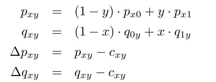
The final value of the reconstructed function is

Extension to four dimensions is straightforward and is shown in Section S4 in the Electronic Supplementary Material(ESM).We apply multi linear interpolation to all sixteen corners of the four dimensional hyper-cubec¯x¯y¯z¯w,where¯x,¯y,¯z,¯w∈{0,1}.Then,values of the slices are interpolated in the three remaining dimensions and the final value of the reconstructed function is computed.

6 Optimal placement of slices

6.1 Basics

Although values along individual slices are measured adaptively,the positions of the slices in BRDF space must be determined in advance.Here we investigate how to place the slices optimally for a given number of samples.Due to a lack of available anisotropic BRDF measurements with high angular density and high accuracy,we performed a study on ten materials represented by the state-of-the-art analytical BRDF model of Kurt et al.[20].We selected ten materials,four of them measured in Ref.[21]and fitted in Ref.[20],and the remaining materials came from our own measurements.All of these materials are anisotropic and include fabrics,brushed aluminum,and untreated wood.Their fitted BRDFs are shown in Fig.5 and the model parameters are included in Section S2 in the ESM.

6.2 Placement theory

The axial and diagonal slices are placed into 2D subspaces selected byθiandθv.The most straightforward approach is to deploy the slices regularly into the subspaces using:

α,β∈{kas;k∈{0,...,an−1},an=2π/as}whereanis the number of slices of one type in one subspace andasis theazimuthal stepbetween two consecutive slices.The single parameterashas to be chosen.While the positions of the axial and diagonal slices might be chosen arbitrarily,for simplicity,we limit ourselves to regular distribution of both types of slices using a common step parameter.

Similarly,2D subspaces are selected by a single parameter,theelevation step es:

Fig.5 Ten test materials represented by the BRDF model in Ref.[20],rendered on spheres,with visualizations of their BRDFs.

whereen=「θmax/es」+1 is the number of elevations used andθmaxis the maximal elevation.Measured subspaces are those resulting from all combinations ofθi,θv.Finally,horizontal and vertical slices are placed through every intersection of the axial and diagonal slices(see Fig.2).

6.3 Analysis of optimal placement

We performed an experiment to determine the optimal positions of the slices based on a user chosen number of samplesn.We used all ten BRDFs of the ten materials(Fig.5)and computed reconstructions of these BRDFs for various combinations ofazimuthal step as,elevation step es,and number of samplesn.To make the precalculation computationally feasible,we restricted the resolution of the reconstructed BRDFs to 2°and we used a maximal elevation angleθmax=80°due to unstable fi tting of the BRDF by the analytical model for high elevation angles.Values of theazimuthal stepparameter wereas∈{12°,20°,36°,60°,180°},and values of theelevation stepparameter werees∈{6°,8°,10°,12°,14°,16°,20°,28°}.In total,we performed 20,646 simulated measurements and reconstructions of BRDFs,which consumed over 20 days of computation time using four cores on an Intel Xeon E5-2643 3.3GHz processor.

To evaluate the quality of the reconstructed BRDFs,we computed the mean relative error(MRE)between the reference BRDFfr(θi,θv,ϕi,ϕv)and its reconstruction(θi,θv,ϕi,ϕv):

whereN=|λ|×|θi|×|θv|×|ϕi|×|ϕv|is the number of data points andλ∈{R,G,B}is a color channel.Individual color channels are treated separately and the results summed. We express MRE as a percentage.

We computed graphs of MRE as a function of the number of adaptive samplesn.This resulted in|as|×|es|×|m|=5×8×10=400 graphs of errm,as,es(n),wheremstands for one of 10 materials.Each graph captures the reconstruction error for a large range of samplesn.Figure 6 plots some of those graphs averaged across all the materials.The first group of graphs in Fig.6(a)shows the error on fi xingthe parameteres=14°and varying the parameteras.The second group of graphs in Fig.6(b)shows the error when fi xing the parameteras=20°and varying the parameteres.The fast convergence of the individual graphs con fi rms the efficiency of the adaptive sampling algorithm.

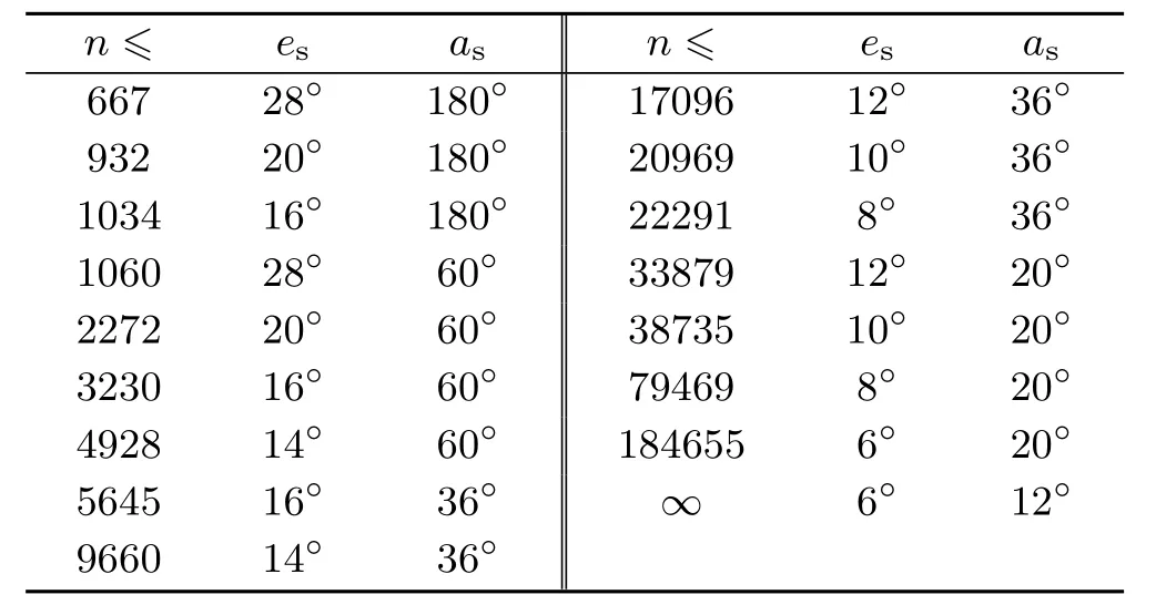
Table 1 Optimal values of the parameters as,esfor various chosen numbers of samples

Fig.6 MRE of the reconstructed BRDF as a function of the number of samples,averaged across all materials(a)for five values of the azimuthal step with a fixed value of es=14°and(b)for eight values of the elevation step with a fixed value of as=20°.

From the graphs,it is possible to conclusively select the best combination of the parametersasandesfor a selected number of samplesn,for a given materialm.Unfortunately,these values differ according to material,as each exhibits individual behavior with respect to changes in the azimuthal and elevation angles.Therefore,we select optimal values^as,^esof these parameters for a given number of samplesnso that the sum of errors across all materials relative to the achievable error is minimized using

The resulting optimalvalues foras,esare summarized in Table 1;when a new material is measured,one should select appropriate values of the parameters for the chosen number of samples.

7 Results

This section presents results of using the proposed method.Firstly,due to lack of reliable data,we use synthetic data generated by the BRDF model(see Fig.5).Thus,we can easily and quickly obtain a BRDF value in any direction and results of the experiment are not influenced by errors caused by a measurement process.To evaluate the method on real data,we used a 3D scene(see Fig.11)and measured all data needed to visualize the scene using a gonioreflectometer. Finally,we compare our method with the previous adaptive method in Ref.[2].

7.1 Simulated measurement experiment

We evaluated accuracy of the proposed method in comparison to use of uniformly distributed samples,taken in directions according to one of the thirty sampling schemes we designed(see Fig.7 and Section S1 of the ESM).These schemes produced in total fromn=435 ton=354,061 reciprocal samples.Values of the samples were interpolated using barycentric[14]or RBF[5]interpolation.Note that the second method is global while the first is local,and is therefore suitable for fast rendering on a GPU.Both methods compute results for each color channel separately.We interpolated the BRDF to a four-dimensional array using a uniform step of 2°and a maximal elevation of 80°,so the dimensions of the array were|θi|×|θv|×|ϕi|×|ϕv|=41×41×180×180.Note that the error values can be compared only for the given number of samples as the barycentric and RBF interpolation methods operated on the 30 predefined sampling schemes. The average MRE(over all materials and schemes)for barycentric interpolation was almost 7.5 times as large as for the BRDF slices.RBF interpolation was better,but its average MRE was still almost 3.9 times as large as for the BRDF slices.

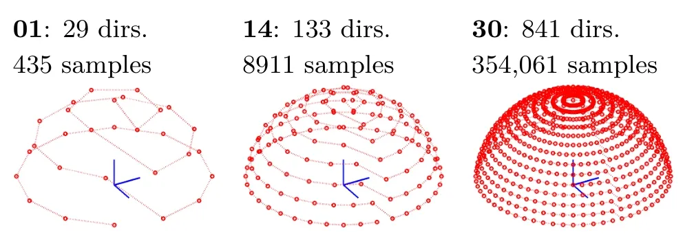
Fig.7 Three of thirty sampling schemes used for uniform sampling of the hemisphere in conjunction with the barycentric and RBF based methods.

Figure 8 shows reconstruction error as a function of the number of samples for all tested methods,for two materials(for other materials see Section S3 of the ESM).Convergence of the proposed algorithm to low MRE values as the number of samples increases is very fast(see the green line in Fig.8).While the RBF method performs well for lower number of samples,the proposed method has better accuracy for higher number of samples.With more than 5000 samples,our method achieves high quality results that are significantly better than those achieved using uniform interpolation methods.

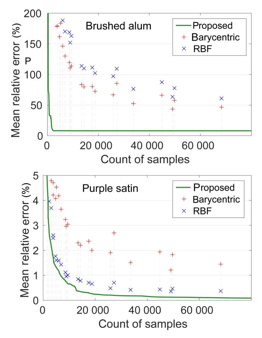
Fig.8 MRE as a function of the number of samples for two materials.

To evaluate quality of the reconstructed BRDF,we computed the MRE between the reference BRDF and its reconstruction atN= 3×41×41×180×180=163,393,200 data points.Improvement in the MRE due to usage of the proposed method instead of barycentric or RBF interpolation for sampling schemes 14(8911 samples)and 19(18,721 samples)is shown in Fig.9.In Fig.10,we compare all three methods with a reference rendering for three materials and 8911 reciprocal samples.We used thegraceenvironment represented by means of 256 lights. (Results for additional materials are shown in Section S3 in the ESM.)The results achieved show that our method provides the best reproduction of the specular reflections and the anisotropic highlights.

7.2 Practical measurement experiment

The previous experiment was performed using reference BRDFs represented by an analytical model.However, such an approach sacrifices some visual features of the original reflectance behavior that cannot be reliably represented by the model. Therefore, we performed practical BRDF measurement experiments,collecting 8911 samples. Firstly, we recorded these samples uniformly(using sampling scheme 14,see Fig.7 and Section S1 of the ESM)and interpolated them using barycentric and RBF methods.Then,we recorded the same number of samples adaptively using our proposed method.Altogether, we measured two datasets for each of three materials(fabric112,fabric135,fabric136)publicly available at http://btf.utia.cas.cz.

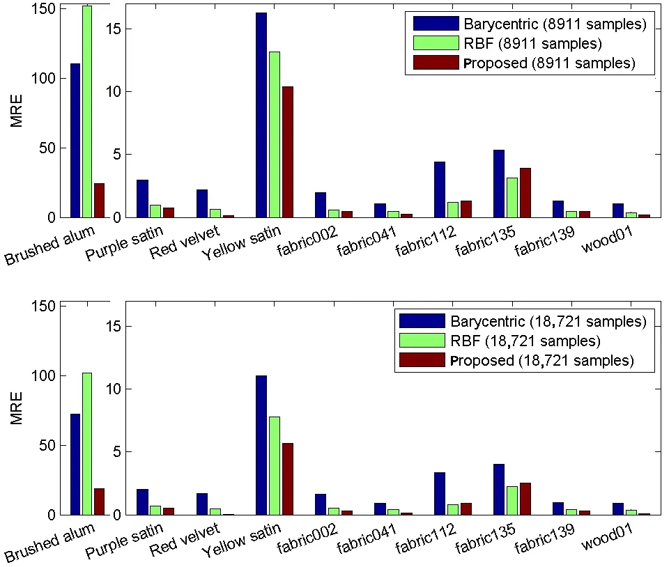
Fig.9 MRE of the proposed method,barycentric interpolation,and RBF interpolation.Top:for sampling scheme 14(8911 samples).Bottom:for sampling scheme 19(18,721 samples).

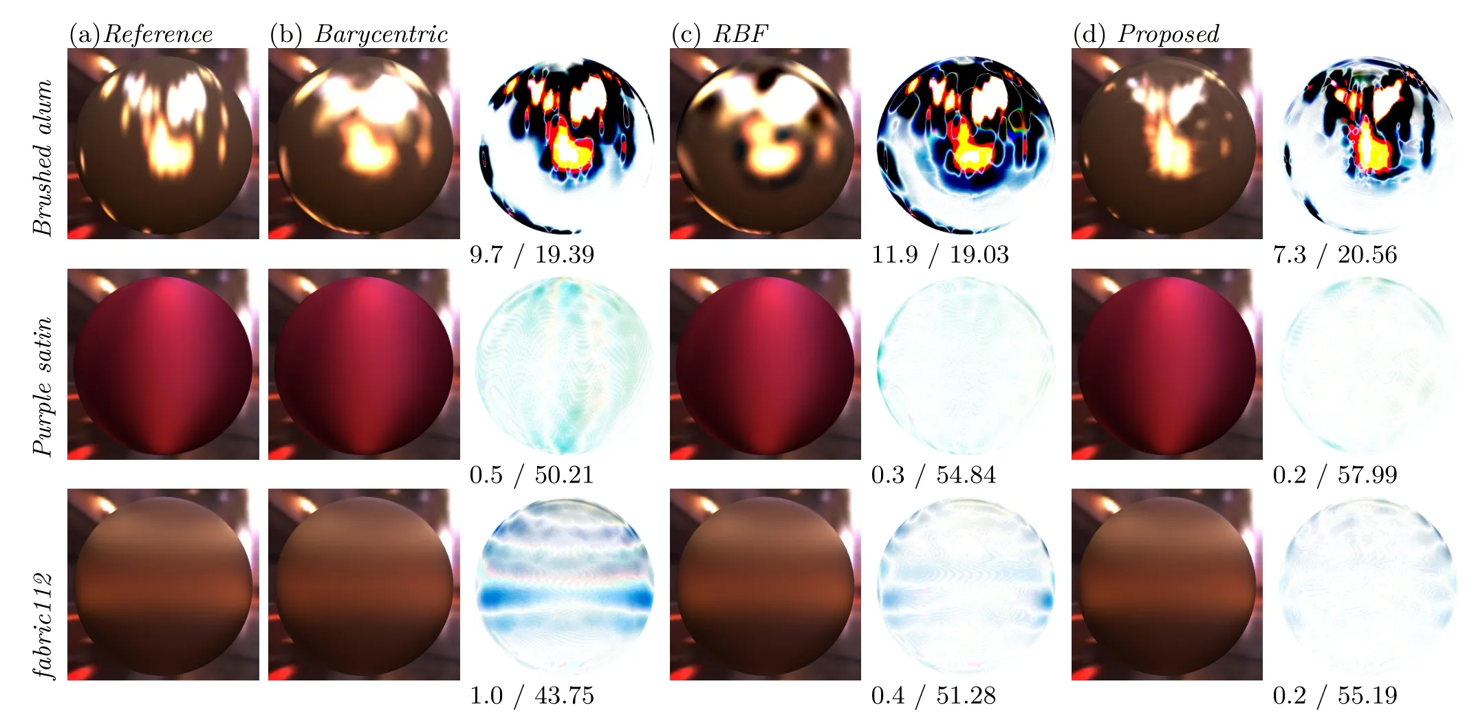
Fig.10 BRDF rendering on a sphere in the grace environment.The reference BRDF(a)is compared with its reconstruction from 8911 samples using(b)barycentric interpolation,(c)RBF interpolation,and(d)our proposed method.Difference images are scaled 10× and difference values are given as CIE ∆E/PSNR(dB).

All measurements were performed using the UTIA gonioreflectometer[2]that allows for the placement of an almost arbitrary combination of illumination and viewing directions with high angular accuracy.Acquisition time for the adaptive method was about 10%longer than for uniform sampling of the same number of samples due to the data processing overhead required by the adaptive algorithm.It took approximately 25 hours to acquire 8911 samples.

We compared the data in an applied situation using a 3D scene comprised offourspheres illuminated by a single point-light source as shown in Fig.11.

Therefore,many combinations of illumination and view directions were covered providing a comprehensive visualization of the properties of these materials.The rendered images were divided into as parseraster with only 6195 occupied pixels representing the directions reachable by the goniore fl ectometer;therefore,only this number of BRDF values was measured for the three materials.

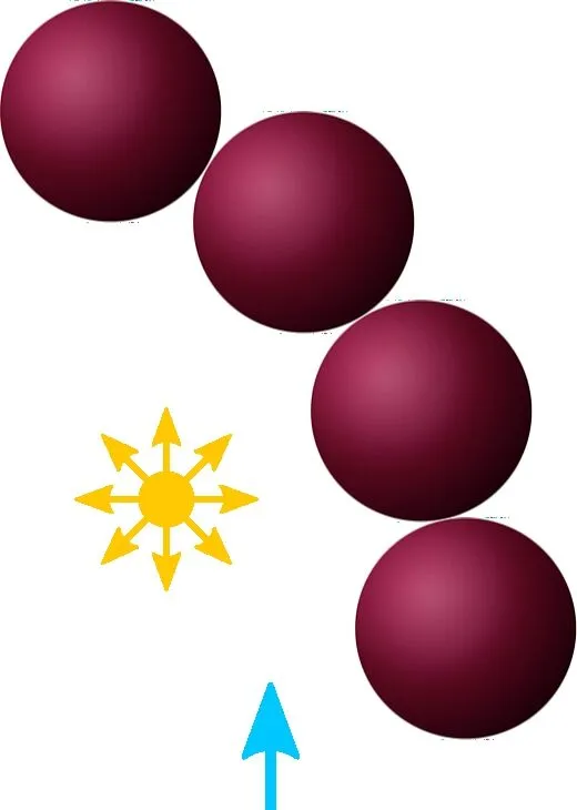
Fig.11 3D scene used for tests on real measured BRDF data.

The entire scene was then rendered using those pixels,which we callcontrol samples;we used them as our reference. Note that pixels representing directions unreachable by the gonioreflectometer due to occlusion of view of the camera by the light source are not included into thecontrol samples(resulting in a white spot in the difference images in Fig.12,on the leftmost sphere).Their values were interpolated from regular measurements for purposes of visualization.

The insufficient precision of analytical models,and also of non-adaptive measurement,is shown by our experiment in Fig.12.Renderings using tabulated data(rows 2,3,and 4)outperform analytical models(rows 5 and 6)in terms of precision. Therefore,tabulated functions should be used whenever high accuracy is important.

We also rendered the same scene using values obtained by the three methods to be compared and evaluated their results at allcontrol samples.Figure 12 shows the reference scene side-by-side with its reconstruction using all tested methods as well as results of two tested analytical anisotropic models due to Kurt et al.[20]and Ward[22].From the accompanying error values,we conclude that our method has by far the best accuracy for real BRDF data.

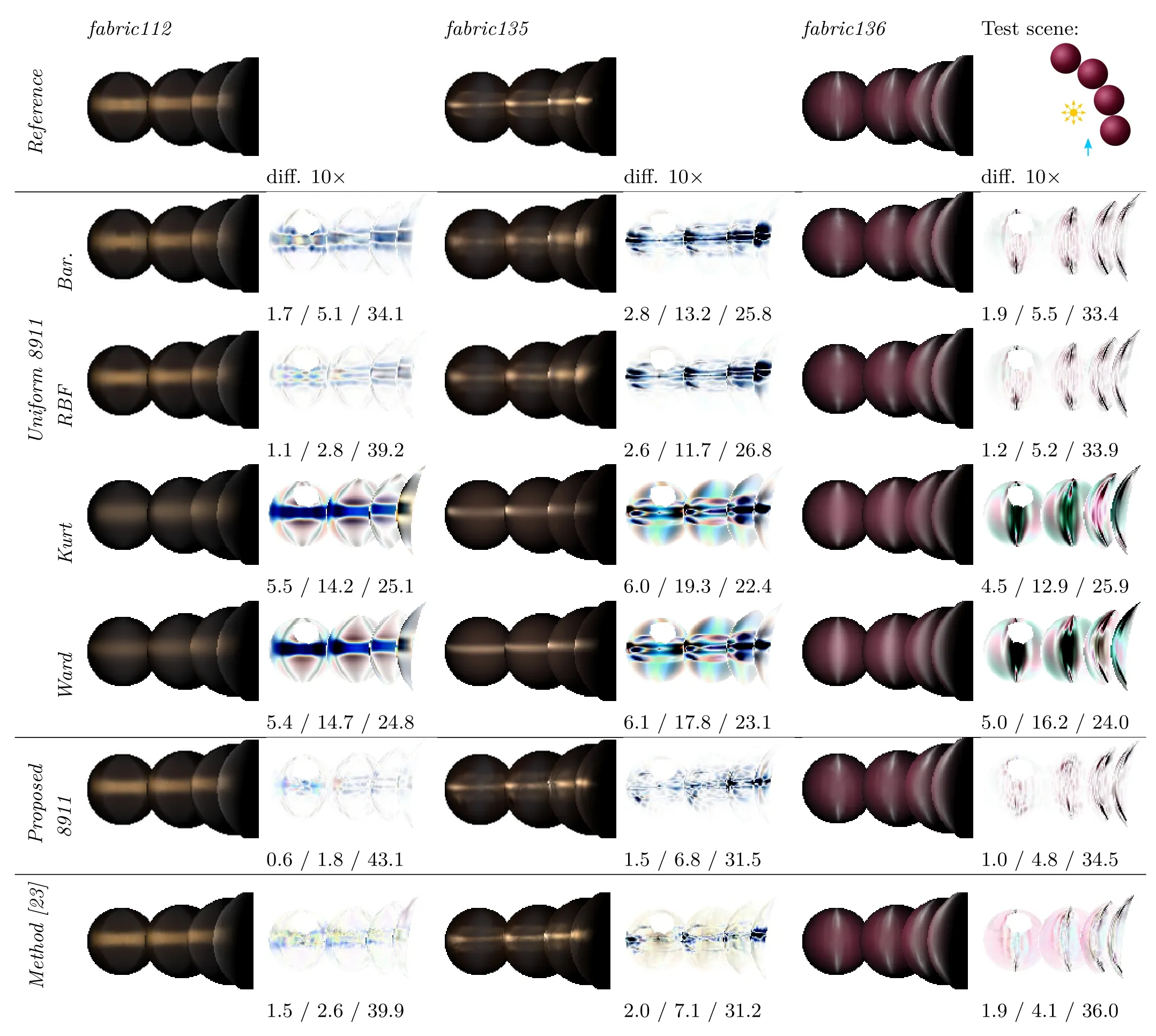
Fig.12 All reachable directions in the virtual scene(see Fig.11)measured and compared with barycentric and RBF interpolations of uniformly measured data, fi ts of two analytical models([20,22]),and our proposed adaptive measurement.8911 samples were used.Difference values are given as CIE∆E/RMSE/PSNR(dB).The last row shows results of dense BRDF measurement[23].

In addition,we show how our method compares to an approach to dense BRDF measurements in Ref.[23].It relies on spatial homogeneity of measured material and slight variations of illumination and viewing angles within each captured image.A total of 8505 images capture nearly three million BRDF samples.After interpolation of missing samples,the data are uniformly resampled with a sampling step of 2°in all four dimensions;these data currently represent one of the best anisotropic BRDF datasets available.The last row of Fig.12 uses such data performance for our test scene,giving difference images and CIE∆E,RMSE,and PSNR values.

When compared to the proposed method(using 8911 samples)in the previous row,one can observe the comparable accuracy of both methods,but while the sequential measurement time for over 8000 images is comparable,the proposed method does not assume largely homogeneous material with the associated challenges related to sample preparation.

7.3 Comparison with a previous adaptive method

We have compared our method with the method of Filip et al.[2]using synthetic data and our own reimplementation of that method. Its results were much worse than ours when we use 12 axial and 12 diagonal slices per subspace as suggested in Ref.[2].Moreover,its parametertmust be tuned carefully to achieve the chosen number of samples,which would not be possible in a real measurement scenario.Thus,we have also enhanced the method with our approach to adaptive sampling(see Section 4)which enables us to choose the number of samples easily.Also,we have taken our conclusions on the optimal placement of samples(see Section 6)into account,which helps greatly.This allows us to evaluate the additional contribution due to the horizontal and vertical slices over and above that of the axial and diagonal slices.Results of the comparison are summarized in Fig.13.Our method on average has only about half the error of even the enhanced version of the method of Filip et al.[2].

7.4 Validation on specular anisotropic materials

Finally, we validated ourmethod on several highly specular anisotropic materials. As such ground truth measurements are not available with sufficient angular density,we have to rely on an anisotropic BRDF model again.We selected three highly reflective self-adhesive aluminum foils with directional finishing. We captured their BRDFs uniformly using 81 samples per hemisphere[24]and fitted this data using an anisotropic BRDF model[20].Photographs of the foils and the captured BRDFs are shown in Fig.14.

The fitted BRDF model was used to generate dense ground truth data for testing of the compared methods. Figure 15,last column,shows that the proposed method clearly performs better than uniform sampling with barycentric or RBF interpolation.One can observe the contribution of the proposed method in comparison to its variant without horizontal and vertical slices[2].

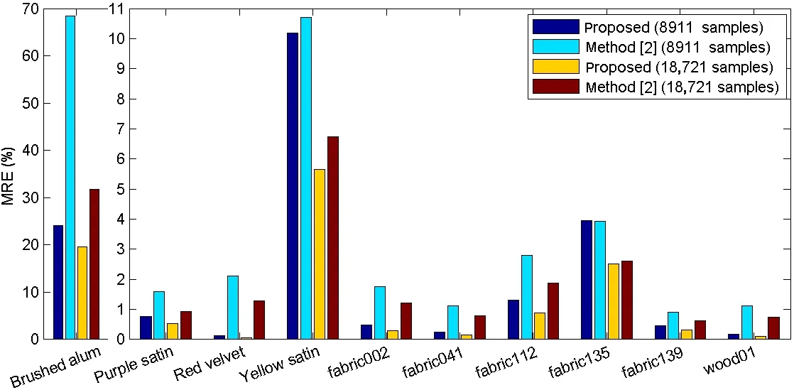
Fig.13 Percentage MRE for the proposed method and the method in Ref.[2]for two numbers of samples(schemes 14 and 19).

Fig.14 Photographs of brushed aluminum samples and corresponding captured BRDFs.

Fig.15 Renderings of three specular anisotropic materials using different sampling approaches and 8911 samples,compared with the ground truth(GT).The difference images are scaled.

Similar results are obtained for the two sampling schemes when the MREs are computed between the ground truth and the values reconstructed by the tested methods,as shown in Table 2. Also see additional results in Section S6 of the ESM.

8 Discussion

This section discusses advantages and limitationsof the proposed method,and gives timings for the interpolation methods used.Furthermore,we discuss reliability of the proposed approach that finds the optimal placement of the slices.

Table 2 MRE of the compared methods for two numbers of samples(schemes 14 and 19)

8.1 Advantages

In contrast to competitive methods,the main advantage ofourproposed adaptive sampling approach is its faster decrease in reconstruction errors with increasing number of samples(especially for lower counts,see Fig.6).On average,we achieve almost four times lower relative errors given the same number of samples,and between two to five times fewer samples are necessary to achieve the same reconstruction errors. Additionally,the proposed adaptive sampling method operates along the one dimensional slices in the BRDF space,allowing data acquisition by continuous movement of a light source and a sensor.It is especially beneficial for accurate gonioreflectometer-based measurement devices.

8.2 Limitations

Common to all tested methods is their decreasing improvement in accuracy as increasing number of samples,approaching an asymptotic value. One reason for this behavior is lack of samples at locations representing specular and anisotropic highlights.They are not sampled properly by the uniform sampling used in the RBF and barycentric methods,nor by the uniform positioning of the slices in BRDF subspaces by the proposed method. We believe that the development of a better parameterization in combination with an adaptive placement of the slices would further improve performance.

As the proposed method is particularly designed to represent features perpendicular to the slices,it can suffer from improper representation of curved highlights or visual features occurring between the slices.Such behavior is typical for subspaces with a large difference between viewing and illumination elevation angles,as shown in Fig.16.These errors can be suppressed by an elevation-angle dependent interpolation method[25]that interpolates data along the anisotropic highlights.Unfortunately,this method is not yet elaborate enough to reconstruct the whole 4D BRDF space.

8.3 Timings

Fig.16 Example of a limitation of the proposed interpolation method,when highlights are not perpendicular to the axial or diagonal slices(θi=30°,θv=75°).

Reconstruction of the entire BRDF space with a uniform step of 2°requires about 45 seconds using barycentric interpolation, whereas RBF interpolation takes about22 minutes; neither depends on the number of samples.Reconstruction of the whole BRDF array by the proposed method using our MATLAB implementation typically takes 4 minutes. All timings were obtained using a single core of an Intel Xeon E5-2643 at 3.3 GHz.Implementation of the method for interpolation of an arbitrary value on a GPU is described in Section S5 of the ESM.

8.4 Stability of placement of slices

To test stability of the proposed placement optimization, we performed the following experiment.We computed the optimal values of the parametersmtimes using Eq.(3),each time with one material left out of the computation.This providesmdifferent results,which we graphically compare in Fig.17 to the results in Table 1.The first line in Fig.17 corresponds to the computation for all materials,and each other line corresponds to the computation with one material left out.

Fig.17 Top row:The color coded optimal placement of slices in terms of es/asfor various numbers of samples.Other rows:Stability test of optimal placement of slices:in each row,one material is left out from computation of the optimal placement.

As one can see,boundaries of individual regions(representing combinations of parameterses/as)vary slightly but not dramatically.When we leave outRed velvet,there is a green region(14/20)which does not appear on other lines substituting purple(10/36)and blue(8/36)regions.When we leaveBrushed alum,fabric041,orwood01out,the blue region(8/36)is missing.Note that usage of the parameters for neighboring regions leads to only slightly worse reconstruction errors.

We evaluated the increase in MRE due to usage of the optimal placement of the BRDF slices according to Table 1,instead of usage of the best placement for the tested material(which is unknown for a newly measured material). Evaluation was performed across a broad range from 55 samples(resulting from the number of slice intersections in the sparsest con fi gurationes= 28°,as= 180°)to 354,061 samples(resulting from the densest tested uniform distribution of samples across a hemisphere,see Fig.7).Results are summarized in Table 3.While the maximal increase in the error is almost 1.5 times,the average MRE across all materials is only 1.2 times worse than if we use the best possible placement of the slices.We conclude that usage of the optimal placement according to Eq.(3)works well in practice for measurement of an unknown material.

Table 3 Increase in MRE using determined optimal placement of the slices,instead of the best possible placement

9 Conclusions

Ourpaperdealswith efficientsampling and reconstruction of anisotropic BRDFs using a chosen number of samples. Firstly,we sample a fourdimensional dataspace by means of one-dimensional slices,with adaptive density of samples along the slices according to material properties. To find the optimal placement of the slices in the 4D BRDF space,we perform an extensive study on ten materials,and we provide parameters for optimal placement based on the required number of measured samples.

We have compared the accuracy of our method with barycentric and RBF interpolation approaches as applied to 30 uniform sampling schemes with varying numbers of samples.In simulated measurements that use an analytical anisotropic BRDF model as a source of reference data,the proposed method achieves on average almost fourtimes lower reconstruction errors than uniform sampling combined with either of two interpolation methods.Alternatively,for a given reconstruction error,our method requires between two to five times fewer samples than the competing approaches.

In real measurement of the anisotropic BRDFs,our method achieves half the reconstruction error of other approaches,and our further experiments suggest that the captured BRDF data are amongst the best publicly available anisotropic BRDFs.We have also verified that the proposed method performs almost twice as well as a previous adaptive method[2],mainly due to its use of two additional types of BRDF slices. Moreover,the proposed method readily allows reconstruction of a BRDF on a GPU.

In our future work,we plan to enhance the interpolation method proposed in Ref.[25]to eliminate the main disadvantage of our method,reconstruction artifacts.Also,we plan to extend our method to a more time-and resource-efficient measurement of spatially-varying representations such as SVBRDFs or BTFs.

Acknowledgements

This research was supported by Czech Science Foundation grant 17-02652S.

Electronic Supplementary MaterialSupplementary materials including a list oftested sampling schemes, fitted parameters of BRDF models,and addition results for all tested materials are available in the online version of this article at https://doi.org/10.1007/s41095-017-0099-z.

References

[1]Nicodemus,F.E.;Richmond,J.C.;Hsia,J.J.;Ginsburg,I.W.;Limperis,T.Geometrical considerations and nomenclature for reflectance.U.S.Department of Commerce,National Bureau of Standards,1977.

[2]Filip,J.;Vavra,R.;Haindl,M.;Zid,P.;Krupicka,M.;Havran,V.BRDF slices:Accurate adaptive anisotropic appearance acquisition.In:Proceedings of the IEEE Conference on Computer Vision and Pattern Recognition,1468–1473,2013.

[3]Ghosh,A.;Achutha,S.;Heidrich,W.;O’Toole,M.BRDF acquisition with basis illumination.In: Proceedings of the IEEE 11th International Conference on Computer Vision,1–8,2007.

[4]Wang,J.;Zhao,S.;Tong,X.;Snyder,J.;Guo,B.Modeling anisotropic surface reflectance with example based microfacet synthesis.ACM Transactions on GraphicsVol.27,No.3,Article No.41,2008.

[5]Press,W.H.;Teukolsky,S.A.;Vetterling,W.T.;Flannery,B.P.Numerical Recipes in C:The Art of Scienti fi c Computing,2nd edn.Cambridge University Press,1992.

[6]Fuchs,M.;Blanz,V.;Lensch,H.P.;Seidel,H.-P.Adaptive sampling of reflectance fields.ACM Transactions on GraphicsVol.26,No.2,Article No.10,2007.

[7]Lensch,H.P.;Lang,J.;S,A.M.;Seidel,H.-P.Planned sampling of spatially varying BRDFs.Computer Graphics ForumVol.22,No.3,473–482,2003.

[8]Nauyoks,S.E.;Freda,S.;Marciniak,M.A.Dynamic data driven bidirectional reflectance distribution function measurement system.In:Proceedings of the SPIE 9205,Re fl ection,Scattering,and Diffraction from Surfaces IV,920502,2014.

[9]Ward,G.; Kurt,M.; Bonneel,N.Reducing anisotropic BSDF measurement to common practice.In: Proceedingsof the Workshop ofMaterial Appearance Modeling,5–8,2014.

[10]Matusik,W.;P fi ster,H.;Brand,M.;McMillan,L.Efficient isotropic BRDF measurement.In:Proceedings of the 14th Eurographics Workshop on Rendering,241–247,2003.

[11]Nll,T.; Khler,J.; Stricker,D.Robustand accurate non-parametric estimation of reflectance using basis decomposition and correction functions.In:Proceedings of the European Conference on Computer Vision,376–391,2014.

[12]Nielsen,J.B.;Jensen,H.W.;Ramamoorthi,R.On optimal,minimal BRDF sampling for reflectance acquisition.ACM Transactions on GraphicsVol.34,No.6,Article No.186,2015.

[13]Vavra,R.;Filip,J.Minimal sampling for effective acquisition of anisotropic BRDFs.Computer Graphics ForumVol.35,No.7,299–309,2016.

[14]Coxeter,H.S.M.Introduction to Geometry.New York:Wiley,1969.

[15]Bookstein, F.L.Principalwarps: Thin-plate splines and the decomposition of deformations.IEEE Transactions on Pattern Analysis and Machine IntelligenceVol.11,No.6,567–585,1989.

[16]Gortler,S.J.;Grzeszczuk,R.;Szeliski,R.;Cohen,M.F.The lumigraph.In:Proceedings of the 23rd Annual Conference on Computer Graphics and Interactive Techniques,43–54,1996.

[17]Bonneel,N.;van de Panne,M.;Paris,S.;Heidrich,W.Displacement interpolation using Lagrangian mass transport.ACM Transactions on GraphicsVol.30,No.6,Article No.158,2011.

[18]Bilgili,A.;ztrk,A.;Kurt,M.Ageneral BRDF representation based on tensor decomposition.Computer Graphics ForumVol.30,No.8,2427–2439,2011.

[19]Filip,J.Restoring illumination and view dependent data from sparse samples.In:Proceedings of the 21th International Conference on Pattern Recognition,1391–1394,2012.

[20]Kurt,M.;Szirmay-Kalos,L.;Kivnek,J.An anisotropic BRDF model for fi tting and Monte Carlo rendering.ACM SIGGRAPH Computer GraphicsVol.44,No.1,Article No.3,2010.

[21]Ngan,A.;Durand,F.;Matusik,W.Experimental analysis of BRDF models.In:Proceedings of the Eurographics Symposium on Rendering,117–126,2005.

[22]Ward,G.J.Measuring and modeling anisotropic reflection.ACM SIGGRAPH Computer GraphicsVol.26,No.2,265–272,1992.

[23]Filip,J.;Vavra,R.;Havlicek,M.Effective acquisition ofdense anisotropic BRDF.In: Proceedings of the 22nd International Conference on Pattern Recognition,2047–2052,2014.

[24]Sattler,M.;Sarlette,R.;Klein,R.Efficient and realistic visualization of cloth.In: Proceedings of the Eurographics Symposium on Rendering,167–178,2003.

[25]Vavra,R.; Filip,J.BRDF interpolation using anisotropic stencils.Electronic ImagingVol.2016,No.9,1–6,2016.