A NEW ADAPTIVE TRUST REGION ALGORITHM FOR OPTIMIZATION PROBLEMS∗

Zhou SHENG(洲)Gonglin YUAN(袁功林) Zengru CUI(崔曾如)

College of Mathematics and Information Science,Guangxi University,Nanning 530004,China

E-mail:szhou03@live.com;glyuan@gxu.edu.cn;cuizengru@126.com

1 Introduction

Consider the following minimization problem:

where f:Rn→ R is a twice continuously differentiable function.This problem has appeared in many applications in the medical science,optimal control,functional approximation,curvefitting fields,and other areas of science and engineering.Many methods are presented to solve this problem(1.1),including the conjugate gradient method(see[1–8]),the quasi-Newton method(see[9–14]),and the trust region method(see[15–28]).

As is known,the trust region method plays an important role in the area of nonlinear optimization,and is among efficient methods for solving problem(1.1).The trust region methods that was firstly proposed by Powell in[29]used of an iterative structure.At each iterative point xk,a trial step dkwas obtained by solving the following subproblem

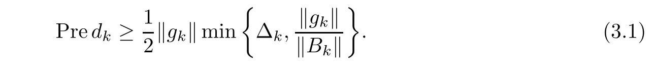
where gk= ∇f(xk),Bkis an n×n symmetric approximation matrix of∇2f(xk),and Δkis the trust region radius.

Solving the trust region subproblem(1.2)plays a key role for solving problem(1.1)in the trust region algorithm.In traditional trust region methods,at each iterative point xk,the trust region radius Δkis independent of the variables gk,Bk,and ‖dk−1‖/‖yk−1‖,where

However,these variables contain first-and second-order information,which we do not use.We determine the initial trust region radius and some artificial parameters to adjust it,and the choice of these parameters has an important in fluence on our numerical results.Therefore,Zhang[25]proposed a modified trust region algorithm by replacing Δkwith,where

and p is a positive integer.With this modified trust region subproblem,instead of updating Δk,p is adjusted.However,at every iteration,we need to calculate the Hessian of f.On the basis of the technique described in[25],Zhang,Zhang,and Liao[19]presented a new trust region subproblem,where the trust region radius usesthe definitions of c,p,gkremain the same as in[25],andis a positive definite matrix based on the Schnable and Eskow[30]modified Cholesky factorization.We see that there are two drawbacks in computing the inverse of the matrixand the Euclidean norm ofat each iterative point xk.Cui and Wu[24]presented a trust region radius by replacing Δkwithwhere µk＞ 0 and satisfies an update rule,and for the same reason as that found by Zhang,Zhang,and Liao[19],this algorithm requires the calculation ofat every iteration.Motivated by the first-and second-order information of gkandLi[26]proposed a modified trust region radius that useswhich confers the advantage of avoiding to computation of the matrixof the inverse andat each iterative point xk.At the same time,it can decrease the workload and computational time involved.However,the algorithm only uses the gradient information.Some authors have also applied adaptive trust region methods to solve nonlinear equations in[31–33].

The purpose of this article is to present an efficient adaptive trust region algorithm to solve(1.1).Motivated by the adaptive technique,the proposed method possesses the following nice properties:(i)the trust region radius uses not only the gradient value but also the function value,(ii)computing the matrixof the inverse and the value ofat each iterative point xkis not required,and(iii)the associated workload and computational time involved are reduced,which is very important for medium-scale problems.

The remainder of this article is organized as follows.In the next section,we brie fly review some basic results of a modified quasi-Newton secant equation and present an adaptive algorithm for solving problem(1.1).In Section 3,we prove the global convergence of the proposed method.In Section 4,we prove the superlinear convergence of the algorithm under suitable conditions.Numerical results are reported in Section 5.We conclude this article in Section 6.

Throughout this article,unless otherwise specified,‖ ·‖ denotes the Euclidean norm of vectors or matrices.

2 New Algorithm

2.1 Modified secant equation

In this subsection,we introduce a modified secant equation.In the general quasi-Newton secant method,the iterate xksatisfieswhere Bkis an approximated Hessian of f at each iterative point and{Bk}satisfies the following secant equation

where dk=xk+1−xk.However,the method is solved by only using the gradient information in(2.1).Motivated by the above observations,we would like Bkto use not only the gradient value information but also the function value information.This problem was studied by some authors.In particular,a modified secant equation was proposed by Wei,Li,and Qi[11];this equation uses both the gradient information and function information.The modified secant equation is defined as

This property holds for all k.

The results of Theorems 2.1 and 2.2 in[11]shows an advantage over(2.1)in this approximate relation,and some authors presented many efficient methods and proven their algorithms to be more effective by replacing ykwith qkin numerical experiments,on the basis of the modified secant equation(see[34–36]etc).

2.2 Algorithmic structure

In this subsection,we present an adaptive trust region method to solve(1.1),which is motivated by the general trust region method and the modified secant equation.We now introduce the trust region method.In each iteration,a trial step dkis generated by solving an adaptive trust region subproblem,in which both the value of the function of f(x)and the value of the gradient of f(x)at xkare used:

where 0＜ c＜ 1,p is a nonnegative integer,Δkis the trust region radius,Bkis generated by the modified BFGS update formula

and Bk+1satisfies the modified secant equation Bk+1dk=qk.

Let dkbe the optimal solution of(2.4).The actual reduction is defined by

and we define the predicted reduction as

Then,we define rkas the ratio between Aredkand Predk

We now list the steps of the new trust region algorithm as follows.

Algorithm 2.1

Step 1Given x0∈ Rnand the symmetric and positive definite matrix B0=I∈ Rn×n,let 0＜ α ＜ 1,0＜ c＜ 1,p:=0,ε ＞ 0 and Δ0:= ‖g0‖.Set k:=0.

Step 2If‖gk‖ ＜ ε,then stop.Otherwise,go to Step 3.

Step 3Solve the adaptive trust region subproblem(2.4)to obtain dk.

Step 4Determine the actual reduction Aredkand the predicted reduction Predkusing(2.6)and(2.7),respectively.Calculate rk=If rk＜ α,then let p:=p+1,go to Step 3;otherwise,go to Step 5.

Step 5Let xk+1:=xk+dk,and compute qk.If＞0,Bk+1is updated by the modified BFGS formula(2.5);otherwise,let Bk+1:=Bk.

Step 6Let k:=k+1,p:=0,and go to Step 2.

Remark 2.1(i)The procedure of“Step 3–Step 4–Step 3”of Algorithm 2.1 is named as inner cycle.

(ii)Suppose that Step 5 of Algorithm 2.1 with Bk+1is updated by the following rules:if＞0 holds,Bk+1is updated by the following BFGS formula

We now give the following lemma.

Lemma 2.1If Bk+1is updated by the BFGS formula(2.5),then＞0 holds if and only if Bk+1inherits the positive property of Bk.

ProofSimilar to the proofs in[32,37],we obtain this result and omit this proof.

3 Convergence Analysis

To establish the global convergence of Algorithm 2.1,we make the following common assumption.

Assumption 3.1

(i)The level set Ω ={x ∈ Rn|f(x)≤ f(x0)}is bounded.

(ii){Bk}is uniformly bounded,that is,there exists a positive constant M＞0 such that

Similar to the famous result of Powell[38],we provide the following lemma.

Lemma 3.1If dkis the solution of(2.4),then

By the definitions of Algorithm 2.1 and Lemma 3.1,one can obtain the following result.

Lemma 3.2Suppose that Assumption 3.1(i)holds,and{xk}is a sequence generated from Algorithm 2.1.Then,for all k,{xk}⊂Ω.

Lemma 3.3Suppose that Assumption 3.1 holds;then,

where pkis the largest p value obtained in internal iterates at current iterate k.

ProofLet dkbe the optimal solution of the trust region subproblem(2.4).It follows from Step 4 of Algorithm 2.1 that we have at the current iteration pointThus,we know thatis a feasible solution of(2.4);then,

This completes the proof.

Lemma 3.4Suppose that we have Aredkand Predkusing(2.6)and(2.7),respectively.Then,we have

ProofBy the definitions of Aredk,Predk,and the Taylor expansion,this is trivial.

The following lemma indicates that“Step 3–Step 4–Step 3”of Algorithm 2.1 does not cycle in the inner loop in finitely.

Lemma 3.5Suppose that Assumption 3.1 holds and that the sequence{xk}is generated by Algorithm 2.1.Then,Algorithm 2.1 is well defined,that is,the inner cycle of Algorithm 2.1 can be left in a finite number of internal iterates.

ProofBy contradiction,suppose that Algorithm 2.1 can not be left in a finite number of internal iterates,that is,Algorithm 2.1 cycles in finitely in“Step 3–Step 4–Step 3”at iterate k.Then,we have

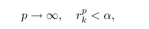
and thus,cp→0 as p→∞.

Therefore,we get

Note that dkis not the optimum solution of(2.4),and it is not difficult to conclude that‖gk‖ ≥ ε.

Now,Lemmas 3.3 and 3.4 lead to

which implies that there exists a sufficiently large p such that

This contradicts the fact that＜ α,which means that Algorithm 2.1 is well-defined,and therefore,the proof is completed.

On the basis of the above lemmas and analysis,we can obtain the global convergence result of Algorithm 2.1 as follows.

Theorem 3.6(Global Convergence) Suppose that Assumption 3.1 holds,and{xk}is a sequence generated from Algorithm 2.1.If ε=0,then Algorithm 2.1 either stops finitely or satisfies

ProofSuppose,on the contrary,that Algorithm 2.1 does not stop.If(3.4)is not true,then there exists a positive constant ε0and an in finite set such that

Because the sequence{f(xk)}is bounded below,we obtain

By Assumption 3.1(ii),there exists a positive constant M such that‖Bk‖ ≤ M for all k,and from Lemma 3.3,we get

where pkis the largest p value obtained in“Step 3–Step 4–Step 3”at iterate xk.Then,we have

Hence,we can assume that pk≥1 for all k∈Γ.

From the definition of pk(k∈ Γ)in“Step 3–Step 4–Step 3”,we know that the solutioncorresponding to the following adaptive trust region subproblem

is unacceptable.

Note that from Lemmas 3.1 and 3.4,we have

Therefore,we obtain

Because pk→+∞as k→+∞,and k∈Γ,we have

This is a contradiction to inequality(3.9).The contradiction shows that(3.4)holds.This completes the proof.

4 Local Convergence

In this section,we will prove the superlinear convergence of Algorithm 2.1 under suitable conditions.

Theorem 4.1(Superlinear Convergence)Suppose that Assumption 3.1 holds,and{xk}is generated by Algorithm 2.1,which converges to x∗and where dkis the solution of(2.4).∇2f(x∗)is positive definite and ∇2f(x)is Lipschitz continuous in a neighborhood of x∗.If the following condition

holds,then Algorithm 2.1 is superlinearly convergent,that is,

ProofBy the definition of dk,from[37],we have

Note that by Theorem 3.6,it is implied that

and thus,we have dk→0.

Consider

where tk∈(0,1).Then,by the property of the norm,we have

Dividing the both sides of the above inequality(4.5)by ‖dk‖,we obtain

Because∇2f(x)is Lipschitz continuous in a neighborhood of x∗,we have

and note that∇2f(x∗)is positive definite.Then,there exist η ＞ 0,k0≥ 0 such that

Hence,we have

Thus,(4.7)implies that

that is,

which means that the sequence{xk}generated by Algorithm 2.1 converges to x∗superlinearly.This completes the proof.

5 Numerical Results

In this section,the numerical results obtained using the proposed method are reported.We call our modified adaptive trust region algorithm NNTR,Zhang’s adaptive trust region algorithm[19]is denoted by ZTR,and Li’s trust region algorithm[26]is denoted by LTR.In the experiments,all parameters were chosen as follows:c=0.5,α =0.1,ε=10−5,and B0=I∈ Rn×n.The parameter for LTR was chosen as c6=0.25.In the tests for NNTR,ZTR,and LTR,we obtain the trial step dkby Steihaug’s algorithm[39]for solving the trust region subproblem(1.2),and to compare the methods,we use the same subroutine to solve the related trust region subproblems.If p≤15 holds,then we will accept the trial step dkin the inner loop“Step 3–Step 4–Step 3”of NNTR,and ZTR.We will also terminate algorithms and consider them to have failed if the number of iterations is larger than 1,200 and 2,500 for small-and medium-scale problems,respectively.All algorithms were implemented in MATLAB R2010b.The numerical experiments were performed on a PC with an Intel Pentium(R)Dual-Core CPU at 3.20 GHz,2.00 GB of RAM and using the Windows 7 operating system.We will test NNTR for both some small-scale problems and medium-scale problems,and compare it with ZTR[19]and LTR[26].

5.1 Specific dimension problems

In this subsection,we list our numerical results for some specific dimension problems(socalled small-scale problems).These problems are listed in Table 5.1,and the test problems can be found in Moré et al[30].In Table 5.1,“No.” denotes the test problem,“Dim” denotes the dimension of problems,“Function” denotes the name of problems,“x0” denotes the initial point, “fopt(x)”refers to the optimum function values,and “–” denotes that the optimum function values are varied.To demonstrate the performance of NNTR for the problems in Table 5.1,we also list the numerical results of ZTR and LTR.The detailed numerical results are reported in Table 5.2,and the following notations are used in Table 5.2: “NI” is the total number of iterations,“NF” is the number of the function evaluations,“f(x)” is the function value at the final iteration,and “fail” is the number of iterations exceeding 1,200,or if the algorithm fails to solve the problem.

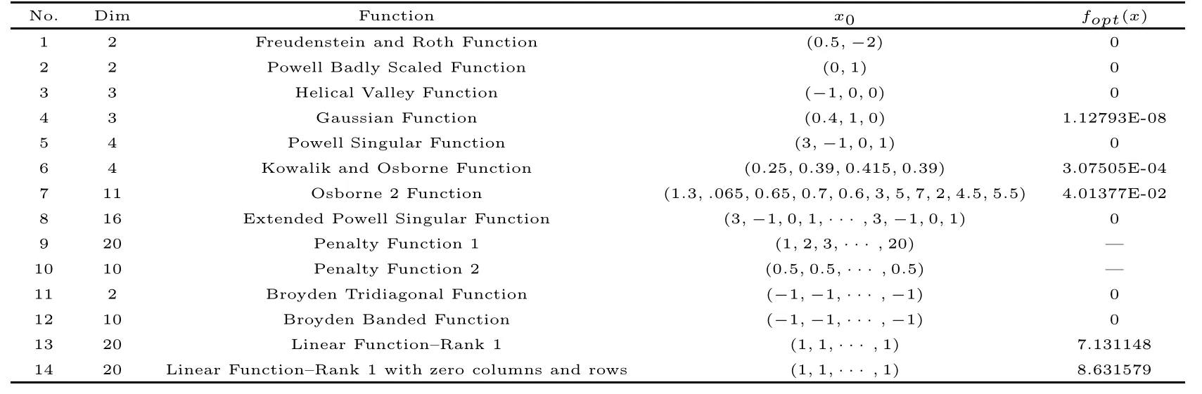
Table 5.1 Problem descriptions for the small-scale testing problems

Remark 5.1For problems 13 and 14 in Table 5.1,we use n=m=30 in all experiments.From Moré[40],we know that the optimum function values areandfor functions 13 and 14,respectively.

Table 5.2 Test results for the small-scale problems

From Table 5.2,we see that the performance of NNTR is better than that of ZTR and LTR for the problems in Table 5.1.Dolan and Moré[41]provided a new tool to analyze the efficiency of these algorithms,where P(t)is the(cumulative)distribution function of the performance ratio.Figures 1 and 2 show that the performance profiles of these algorithms correspond to those of NI and NF,respectively,in Table 5.2 for the small-scale problems in Table 5.1.These two figures show that the NNTR has a good performance for all the problems,when compared it with the ZTR and LTR.

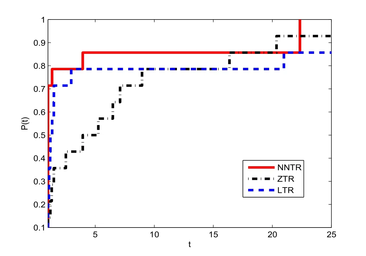
Figure 1 Performance profiles of the methods for these small-scale problems(NI)

Figure 2 Performance profiles of the methods for these small-scale problems(NF)

5.2 Variable dimension problems

Numerical results are reported for some variable dimension problems whose dimension n is chosen in the range[30,1500](so-called medium-scale problems)in this subsection.We list these problems in Table 5.3,and these test problems can be found in Andrei[42].The columns in Table 5.3 are similar to those in Table 5.1.Similar to the numerical results of the smallscale problems,to demonstrate the performance of NNTR for these problems in Table 5.3,the detailed numerical results of NNTR,LTR,and ZTR are listed in Tables 5.4,5.5,and 5.6.The notations in Tables 5.4,5.5,and 5.6 are also similar to those in Table 5.2.It is worth noting that “fail” indicates either the number of iterations exceeding 2,500 or that the algorithm fails to solve the problem,“CPU time” represents the CPU time in seconds required to solve the problem,and “‖g(x)‖” indicates norm of the final gradient.

Table 5.3 Problem descriptions for some testing problems

Table 5.4 Test results for these problems with NNTR

Table 5.5 Test results for these problems with LTR

Table 5.6 Test results for these problems with ZTR

Table 5.7 The sum of NI,NF,and CPU time in Tables 5.4,5.5,and 5.6

Figure 3 Performance profiles of the methods for these problems(NI)

Figure 4 Performance profiles of the methods for these problems(NF)

Figure 5 Performance profiles of the methods for these problems(CPU time)

For these problems,from Tables 5.4,5.5,and 5.6,we know that the performance of NNTR is overall the best among the three algorithms.The NI and NF of ZTR are less than those of NNTR in problems 6,7,31,37-39,44,46,47,and 68-70;however,the CPU time required is larger than that for NNTR.In particular,we see that the total values of NI,NF,and CPU time of NNTR are less than those for LTR and ZTR from Table 5.7,and the difference is significant,about 6332.78 s and 52664.86 s,respectively,for solving all of the test problems in Table 5.3.Moreover,we see that subject to the CPU time metric,NNTR is the top performer.We used the performance profiles that Dolan and Moré[41]used to compare these algorithms again.Figures 3,4,and 5 show that the performance profiles of these algorithms are comparable to the values of NI,NF,and CPU time,respectively,in Tables 5.4,5.5,and 5.6 for the mediumscale problems in Table 5.3.These three figures show that NNTR has a good performance for all problems compared with LTR and ZTR.

6 Conclusions

In this article,using a modified secant equation with the BFGS updated formula and the new trust region radius of the trust region subproblem by replacing Δkwithwe present a new adaptive trust region method to solve optimization problems.

Our method possesses the following attractive properties:(i)the trust region radius uses not only the gradient information but also the function value information,(ii)the adaptive trust region radius is automatically based on dk−1,qk−1,and gk,(iii)the computation of the matrixof the inverse and the value of‖^B−1k‖are not required at each iterative point xk,which therefore reduces the workload and time involved,and(iv)global convergence is established under some mild conditions,and we show that locally,our method shows superlinear convergence.

It is well known that trust region methods are efficient techniques for optimization problems.The numerical results show that the proposed method is competitive with ZTR and LTR for small-scale problems and medium-scale problems with a maximum dimension of 1,500,in the sense of the performance profile introduced by Dolan and Moré[41].We therefore consider the numerical performance of the algorithm to be quite attractive.However,NNTR,ZTR,and LTR fail to solve the test problems at dimensions larger than 2,000 as memory issues with MATLAB.

It would be interesting to test our method’s performance when it is applied to solve nonsmooth optimization problems and some large-scale problems.It would also be interesting to see how the choice of trust region radius affects the numerical results obtained upon solving optimization problems and nonlinear equations with constrained conditions.These topics will be the focus of our future research.

[1]Andrei N.An adaptive conjugate gradient algorithm for lagre-scale unconstrained optimization.J Comput Appl Math,2016,292:83–91

[2]Yuan G.Modified nonlinear conjugate gradient methods with sufficient descent property for large-scale optimization problems.Optim Lett,2009,3:11–21

[3]Yuan G,Lu X.A modified PRP conjugate gradient method.Anna Operat Res,2009,166:73–90

[4]Yuan Lu X,Wei Z.A conjugate gradient method with descent direction for unconstrained optimization.J Comput Appl Math,2009,233:519–530

[5]Yuan G,Wei Z,Zhao Q.A modified Polak-Ribière-Polyak conjugate gradient algorithm for large-scale optimization problems.IEEE Tran,2014,46:397–413

[6]Yuan G,Meng Z,Li Y.A modified Hestenes and Stiefel conjugate gradient algorithm for large-scale nonsmooth minimizations and nonlinear equations.J Optimiz Theory App,2016,168:129–152

[7]Yuan G,Zhang M.A three-terms Polak-Ribière-Polyak conjugate gradient algorithm for large-scale nonlinear equations.J Comput Appl Math,2015,286:186–195

[8]Yuan G,Zhang M.A modified Hestenes-Stiefel conjugate gradient algorithm for large-scale optimization.Numer Func Anal Opt,2013,34:914–937

[9]Zhang H,Ni Q.A new regularized quasi-Newton algorithm for unconstrained optimization.Appl Math Comput,2015,259:460–469

[10]Lu X,Ni Q.A quasi-Newton trust region method with a new conic model for the unconstrained optimization.Appl Math Comput,2008,204:373–384

[11]Wei Z,Li G,Qi L.New quasi-Newton methods for unconstrained optimization problems.Appl Math Comput,2006,175:1156–1188

[12]Yuan G,Wei Z.The superlinear convergence analysis of a nonmonotone BFGS algorithm on convex objective functions.Acta Math Sci,2008,24B:35–42

[13]Yuan G,Wei Z,Lu X.Global convergence of the BFGS method and the PRP method for general functions under a modified weak Wolfe-Powell line search.Appl Math Model,2017,47:811–825

[14]Yuan G,Sheng Z,Wang B,et al,The global convergence of a modified BFGS method for nonconvex functions.J Comput Appl Math,2018,327:274–294

[15]Fan J,Yuan Y.A new trust region algorithm with trust region radius converging to zero//Li D.Proceedings of the 5th International Conference on Optimization:Techniques and Applications(December 2001,Hongkong),2001:786–794

[16]Hei L.A self-adaptive trust region algorithm.J Comput Math,2003,21:229–236

[17]Shi Z,Guo J.A new trust region method for unconstrained optimization.J Comput Appl Math,2008,213:509–520

[18]Shi Z,Wang S.Nonmonotone adaptive trust region mthod.Eur J Oper Res,2011,208:28–36

[19]Zhang X,Zhang J,Liao L.An adaptive trust region method and its convergence.Sci in China,2002,45A:620–631

[20]Zhou Q,Zhang Y,Xu F,et al.An improved trust region method for unconstrained optimization.Sci China Math,2013,56:425–434

[21]Ahookhosh M,Amini K.A nonmonotone trust region method with adaptive radius for unconstrained optimization problems.Comput Math Appl,2010,60:411–422

[22]Amini K,Ahookhosh M.A hybrid of adjustable trust-region and nonmonotone algorithms for unconstrained optimization.Appl Math Model,2014,38:2601–2612

[23]Sang Z,Sun Q.A new non-monotone self-adaptive trust region method for unconstrained optimization.J Appl Math Comput,2011,35:53–62

[24]Cui Z,Wu B.A new modified nonmonotone adaptive trust region method for unconstrained optimization.Comput Optim Appl,2012,53:795–806

[25]Zhang X.NN models for general nonlinear programming,in Neural Networks in optimization.Dordrecht/Boston/London:Kluwer Academic Publishers,2000

[26]Li G.A trust region method with automatic determination of the trust region radius.Chinese J Eng Math(in Chinese),2006,23:843–848

[27]Yuan G,Wei Z.A trust region algorithm with conjugate gradient technique for optimization problems.Numer Func Anal Opt,2011,32:212–232

[28]Yuan Y.Recent advances in trust region algorithms.Math Program,2015,151:249-281

[29]Powell M J D.A new algorithm for unconstrained optimization//Rosen J B,Mangasarian O L,Ritter K.Nonlinear Programming.New York:Academic Press,1970:31–65

[30]Schnabel R B,Eskow E.A new modified Cholesky factorization.SIAM J Sci Comput,1990,11:1136–1158

[31]Zhang J,Wang Y.A new trust region method for nonlinear equations.Math Method Oper Res,2003,58:283–298

[32]Yuan G,Wei Z,Lu X.A BFGS trust-region method for nonlinear equations.Computing,2011,92:317–333

[33]Fan J,Pan J.An improve trust region algorithm for nonlinear equations.Comput Optim Appl,2011,48:59–70

[34]Yuan G,Wei Z,Li G.A modified Polak-Ribière-Polyak conjugate gradient algorithm for nonsmooth convex programs.J Comput Appl Math,2014,255:86–96

[35]Yuan G,Wei Z.Convergence analysis of a modified BFGS method on convex minimizations.Comput Optim Appl,2010,47:237–255

[36]Xiao Y,Wei Z,Wang Z.A limited memory BFGS-type method for large-scale unconstrained optimization.Comput Math Appl,2008,56:1001–1009

[37]Yuan Y,Sun W.Optimization Theory and Methods.Beijing:Science Press,1997

[38]Powell M J D.Convergence properties of a class of minimization algorithms//Mangasarian Q L,Meyer R R,Robinson S M.Nonlinear Programming.Vol 2.New York:Academic Press,1975

[39]Steihaug T.The conjugate gradient method and trust regions in large scale optimization.SIAM J Numer Anal,1983,20:626–637

[40]Moré J J,Garbow B S,Hillstrom K H.Testing unconstrained optimization software.ACM Tran Math Software,1981,7:17–41

[41]Dolan E D,Moré J J.Benchmarking optimization software with performance profiles.Math Program,2002,91:201–213

[42]Andrei N.An unconstrained optimization test function collection.Advan Model Optim,2008,10:147–161