QUALITATIVE ANALYSIS OF A STOCHASTIC RATIO-DEPENDENT HOLLING-TANNER SYSTEM∗
2018-05-05JingFU付静
Jing FU(付静)
School of Mathematics,Changchun Normal University,Changchun 130032,China
E-mail:xibeidaxue232@163.com
Daqing JIANG(蒋达清)1,2,3 Ningzhong SHI(史宁中)1 Tasawar HAYAT2,4 Ahmed ALSAEDI2
1.School of Mathematics and Statistics,Key Laboratory of Applied Statistics of MOE,Northeast Normal University,Changchun 130024,China;
2.Nonlinear Analysis and Applied Mathematics(NAAM)Research Group,Department of Mathematics,Faculty of Science,King Abdulaziz University,Jeddah 121589,Saudi Arabia;
3.College of Science,China University of Petroleum(East China),Qingdao 266580,China
4.Department of Mathematics,Quaid-i-Azam University 45320,Islamabad 44000,Pakistan
E-mail:daqingjiang2010@hotmail.com;shinz@nenu.edu.cn;tahaksag@yahoo.com;aalsaedi@hotmail.com
1 Introduction
The famous Holling-Tanner model which is also known as semi-ratio-dependent Holling type II for predator-prey interaction is expressed in the form:

where N(t)and P(t)represent population densities of the prey and the predator,respectively.Parameters r,s,k,c,and a are positive constants,and represent the growth rate of prey and predator species,the carrying capacity of the prey,capturing rate,and half capturing saturation,respectively.Parameter h>0 is the number of prey required to feed one predator at equilibrium conditions.Recently,more and more mathematicians and biologists have drawn attention on this model and have shown rich dynamical behaviors[1–7].
The traditional prey-predator models with the functional responses depend on prey density only,and are not demonstrated by the data of numerous experiments and observations[8–10].In fact,the predator has to search and compete for food and the ratio-dependent function of the prey and the predator is more suitable to substitute for the model with complicated interaction between the prey and predator.Then,this model is expressed in the form:

subjected to the same conditions as given above.Both theoretical and mathematical biologists studied the ratio-dependent Holling-Tanner model(refer to[8,11–14]).In particular,Liang and Pan[12]analyzed system(1.2)and derived rich dynamical properties.Firstly,they nondimensionalized system(1.2)with the scaling rt→t,→N,→P,and assumed the following conditions:
(A1):αβ+1> β;
(A2):α>1;
(A3):(αβ +2)β < (δβ +1)(αβ +1)2;
(A4):(αβ +2)β > (δβ +1)(αβ +1)2;
(A5):αβ +1 > max{β,},
If condition(A1)holds,then system(1.2)has a unique positive equilibrium E∗(N∗,P∗),where,P∗= βN∗;if condition(A2)holds,then system(1.2)is permanent;if conditions(A1)and(A3)hold,then the positive equilibriumof system(1.2)is locally asymptotical state;if conditions(A1)and(A4)hold,then the positive equilibriumof system(1.2)is an unstable focus or node;If condition(A5)holds,then the positive equilibriumof system(1.2)is globally asymptotical stable in the interior of the first quadrant;If conditions(A1)and(A4)hold,then system(1.2)has a unique limit cycle.
Most of the works on Holling-Tanner or ratio-dependent Holling-Tanner models are in a deterministic environment.May[15]pointed out that because of continuous fluctuations in the environment,the birth rates,the death rates,competition coefficients,and other parameters involved in model(1.2)exhibit random fluctuation to some extent.Recently,The effect of environment on dynamical behaviors of stochastic modified Holling-Tanner model was investigated by Ji[16,17].And for many other articles on the stochastic models,refer to[18–21].In this article,we express system(1.2)with random perturbation in the following form:

Throughout this article,let(Ω,F,{Ft}t≥0,N)be a complete probability space with a filtration{Ft}t≥0.Let Bi(t)(i=1,2)denote the independent standard Brownian motions defined on this probability space.
2 Existence of the Positive Solution
If the coefficients of equation satisfy the linear growth condition and local Lipschitz condition,then the stochastic differential equation has a unique global(that is no explosion in a finite time)solution for any given initial value(see[22]).However,the coefficient of system(1.3)neither satisfy the linear growth condition,nor local Lipschitz continuous.In this section,by making the change of variables and the comparison theorem of stochastic differencial equations,we will show there is a unique global positive solution with positive initial value of system(1.3).
Lemma 2.1There is a unique positive local solution(N(t),P(t))for t∈ [0,τe)of system(1.3)a.s.for any initial value N0>0 and P0>0.
ProofFirstly,we transform system(1.3)into the following equivalent form

on t≥ 0 with initial value u(0)=lnN0,v(0)=lnP0.Obviously,the coefficients of Equation(2.1)satisfy the local Lipschitz condition,then there is a unique local solution(u(t),v(t))on t ∈ [0,τe),where τeis the explosion time(see[28]).By It’s formula,it is easy to see that N(t)=eu(t),P(t)=ev(t)is the unique positive local solution to equation(1.3)with initial value N0>0 and P0>0.
From Lemma 2.1,we know that there is a unique positive local solution of system(1.3).Subsequently,we prove that this solution is global,that is,τe= ∞.We consider the following auxiliary stochastic differential equations:

with the initial value Φ(0)= φ(0)=N0and Ψ(0)= ψ(0)=P0.The solutions of equations(2.2)and(2.3)are written as

Using the comparison principle of stochastic differential equation,we have

From the process of solution Φ(t),φ(t),Ψ(t),ψ(t),it is clear that these solutions are well defined for all t∈ [0,∞)a.s.Thus,we obtain
Theorem 2.2For any given initial value(N0,P0)∈,there is a unique positive global solution(N(t),P(t))of equation(1.3)for t≥0 a.s.Meanwhile,there exist the functions Φ(t),φ(t),Ψ(t),and ψ(t)such that φ(t)≤ N(t)≤ Φ(t)and ψ(t)≤ P(t)≤ Ψ(t),t≥ 0.
3 The Long Time Behavior of System(1.3)
3.1 Persistence
In this part,we assume that
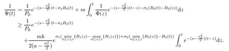
Let Φ(t)and φ(t)are solutions of systems(2.2),by the similar approach in Lemma A.1 of Ji[23],under the conditionwe obtain

and

This and(2.6)imply that

and

Theorem 3.1Under the condition(H),for any initial value(N0,P0)∈,the solution N(t)of system(1.3)is persistence in mean.We have

Next,using a series of operations and the strong law of large numbers(Ji[23,page 1332–1333]),one has

and

On the other hand,from Ji[23](page 1331),we know

therefore,
Subsequent proof is similar to Lemma A.1(page 1339)of[23],then it yields

Consequently,

Combining(3.2)and(3.3),we have

Besides,by Itˆo’s formula,system(1.2)is written as

Integrating from 0 to t,then dividing by t on both sides of(3.4),it yields

Letting t→∞,we obtain
Theorem 3.2The solution(N(t),P(t))of system(1.3)for any initial valuehas
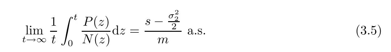
In addition,with the decreasing intensity of the white noise,we take note that the value of(3.5)converges to the valuein the meaning of time average.In this context,it means that stochastic perturbation does not change the permanence of the deterministic system.
Definition 3.3System(1.3)is said to be persistence in mean,if
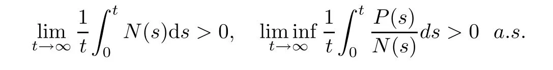
From(3.5),we directly have
Theorem 3.4System(1.3)is said to be persistence in mean,if condition(H)hold.
3.2 Extinction
We know that the establishment of the persistence of system(1.3)depend on condition(H).Supposing that condition(H)is not satisfied,what then?
Theorem 3.5Let(N(t),P(t))be the solution of system(1.3)for any initial value(N0,P0)∈R2+,then,
ProofThe proof is standard and hence is omitted(see Section 3 of[16]).We also obtain the prey and the predator are all extinct ifand
4 Stationary Distribution and Ergodicity for System(1.3)
In this section,our object is to investigate the conditions of the existence of a unique stationary distribution of system(1.3).It is useful to prepare some knowledge to prove the theorem in this part(see Section 2 in[17]).
Let X(t)be a homogeneous Markov process in En⊂Rndescribed by the following stochastic differential equation:
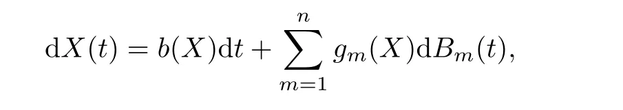
Lemma 4.1(see[24])We assume that there exists a bounded domain D⊂Enwith regular boundary Γ,having the following properties:
(B.1)In the domain D and some neighborhood thereof,the smallest eigenvalue of the diffusion matrix A(x)is bounded away from zero;
(B.2)if x ∈ EnD,the mean time τ at which a path issuing from x reaches the set D isfinite,andfor every compact subset k⊂En.
Then,we have the following result:
The Markov process X(t)has a stationary distribution µ(·),for any integrable function f(·)in regard to the measure µ,that is,

Remark 4.2The proof is given in[24].The existence of stationary distribution with density is referred to Theorem 4.1,p.119 and Lemma 9.4,p.138.The weak convergence and the ergodicity are obtained in Theorem 5.1,p.121 and Theorem 7.1,p130.
To validate(B.1),it suffices to prove that F is uniformly elliptical in any bounded domain D,wherethat is,there is a positive number M such that(see Chapter 3,p.103 of[24]and Rayleigh’s principle in[25,Chapter 6,p.349]).To validate(B.2),it is enough to show that there exists some neighborhood D and a non-negative C2-function V such that LV is negative for any EnD(details refer to[26,p.1163]).
Theorem 4.3If condition(H)holds,then for any initial value(N0,P0)∈R2+,(N(t),P(t))of system(1.3)has a unique stationary distribution µ(·)and it is ergodic.
ProofFirstly,system(1.3)can be expressed by the following form

and the diffusion matrix is


which implies condition(B.1)is validated.Next,we need to verify condition(B.2)in Lemma 4.1.
Define a C2-function V:→R+by

where N and P are also the positive solution of(1.3)for any initial value(N0,P0),and it is satisfied for k thatWe find(1,k)is the minimum point of(4.1),here V(1,k) > 0.It is verified that V(N,P)is nonnegative.By Itˆo’s formula,we calculate
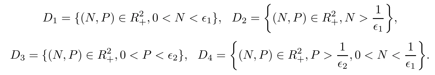
Consider the bounded set

then

here,
We choose sufficiently small∈1,∈2and ∈2=such that
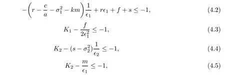
where K1and K2are defined by(4.6)and(4.7)below.
Case 1When(N,P)∈D1,we have

From(4.2),we obtain LV≤−1.
Case 2For any(N,P)∈D2,we have
where

and in view of(4.3),we obtain LV≤−1.
Case 3If(N,P)∈D3,we have

where

and in view of(4.4),this indicates LV≤−1.
Case 4Supposing(N,P)∈ D4and noticing ∈2= ∈21,then

From condition(4.5),we also obtain LV≤−1.
We can take D to be a neighborhood of the rectangular and define a non-negative C2-function such that LV is negative for anywhich implies condition(B.2)in Lemma 4.1 is satisfied.Therefore,the stochastic system(1.3)has a unique stationary distribution µ(·)and it is ergodic.From Theorem 3.2 and Theorem 4.1,we derive the following theorem.
Theorem 4.4If the condition(H)holds,then for any initial value(N0,P0)∈,the solution(N(t),P(t))of system(1.3)has the property

5 Numerical Simulation and Discussion
With the help of matlab software,our outcomes can be examined by the method mentioned in[27].Consider the discretization equation:

where ξkand ηk(k=1,2,···n)are the Gaussian random variables N(0,1).We obtain the following numerical simulation,through appropriate choice of the parameters.
Firstly,the numerical simulation with environmental intensities σ1=0.02,σ2=0.04 is carried out.Parameters satisfy conditionsaccording with the condition of Theorem 3.1–3.3.In the left of Figure 1,we observe that the population densities fluctuate around the the equilibrium(N∗,P∗)of the deterministic system.Stationary distribution of the prey N(t)and the predator P(t)are provided in the right of Figure 1.

Figure 1 The left pictures express the solutions of systems(1.3)and(1.2)for(N0,P0)=(0.5,0.5),r=0.1,f=0.07,c=0.06,a=1,b=0.1,s=0.51 and m=0.2.The red lines represent the solution(N(t),P(t))of system(1.3),while the blue lines represent the solution(N(t),P(t))of model(1.2),here σ1=0.02,σ2=0.04.The right pictures show system(1.3)has a unique stationary distribution.
We choose intensities of the white noise σ1=0.01,σ2=0.21,thus Case 1 in Theorem 3.4 is satisfied.In Figure 2,we see that the prey is persistent and the predator is extinct.In Figure 3,choosing parameters such thatandwe can observe that the species P(t)is extinct as Theorem 3.3(ii)has said and the N(t)is also going to die.The last figure expresses the prey and the predator are all extinct according with the conditionsandHowever,the corresponding deterministic system is persistent in Figures 2–4.These show that the strong white noise may make a persistent system to be extinct.
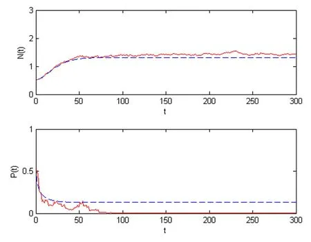
Figure 2 These figures express the solutions of systems(1.3)and(1.2)for(N0,P0)=(0.5,0.5),r=0.1,f=0.07,c=0.06,a=1,b=0.1,s=0.02,and m=0.2.The red lines represent the solution(N(t),P(t))of system(1.3),while the blue lines represent the solution(N(t),P(t))of model(1.2),here σ1=0.01,σ2=0.21.

Figure 3 These figures show the solutions of systems(1.3)and(1.2)for(N0,P0)=(0.5,0.5),r=0.1,f=0.07,c=0.09,a=1,b=0.1,s=0.51,m=0.2.The red lines represent the solution(N(t),P(t))of system(1.3),while the blue lines represent the solution(N(t),P(t))of model(1.2),here σ1=0.5,σ2=0.01.

Figure 4 This group picture illustrates the solutions of systems(1.3)and(1.2)for(N0,P0)=(0.5,0.5),r=0.1,f=0.07,c=0.09,a=1,b=0.1,s=0.02,m=0.2.The red lines represent the solution(N(t),P(t))of system(1.3),while the blue lines represent the solution(N(t),P(t))of model(1.1),here σ1=0.5,σ2=0.21.
[1]Kooij R E,Arus J T,Embid A G.Limit cycles in the Holling-Tanner model.Publicacions Matematiques,1997,41:149–167
[2]Wang M,Pang P Y H,Chen W.Sharp spatial patterns of the diffusive Holling-Tanner prey-predator model in heterogeneous environment.Ima Journal of Applied Mathematics,2008,73(5):815–835
[3]Peng R,Wang M.Global stability of the equilibrium of a diffusive Holling-Tanner prey-predator model.Applied Mathematics Letters,2007,20(6):664–670
[4]Braza P A.The bifurcation structure of the Holling-Tanner model for predator-prey interactions using two-timing.Siam Journal on Applied Mathematics,2003,63(3):889–904
[5]Li J,Gao W.A strongly coupled predator-prey system with modified Holling-Tanner functional response.Computers Mathematics with Applications,2010,60(7):1908–1916
[6]Hsu S B,Huang T W.Global stability for a class of predator-prey systems.Siam Journal on Applied Mathematics,1995,55(3):763–783
[7]Li X H,Lu C,Du X F.Permanence and global attractivity of a discrete semi-ratio-dependent predatorprey system with Holling IV type functional response.Journal of Mathematical Research with Applications,2010,30(3):442–450
[8]Arditi R,Saiah H.Empirical evidence of the role of heterogeneity in ratio-dependent consumption.Ecology,1992,73(5):1544–1551
[9]Arditi R,Ginzburg L R,Akcakaya H R.Variation in plankton densities among lakes:a case for ratiodependent predation models.American Naturalist,1991,138(5):1287–1296
[10]Gutierrez A P.Physiological basis of ratio-dependent predator-prey theory:the metabolic pool model as a paradigm.Ecology,1992,73(5):1552–1563
[11]Arditi R,Ginzburg L R.Coupling in predator-prey dynamics:ratio dependence.Journal of Theoretical Biology,1989,139(3):311–326
[12]Liang Z,Pan H.Qualitative analysis of a ratio-dependent Holling-Tanner model.Journal of Mathematical Analysis Applications,2007,334(2):954–964
[13]Saha T,Chakrabarti C.Dynamical analysis of a delayed ratio-dependent Holling-Tanner predator-prey model.Journal of Mathematical Analysis Applications,2009,358(2):389–402
[14]Banerjee M,Banerjee S.Turing instabilities and spatio-temporal chaos in ratio-dependent Holling-Tanner model.Mathematical Biosciences,2012,236(1):64–76
[15]Fellowes M.Stability and complexity in model ecosystems.Biologist,2001
[16]Ji C,Jiang D,Shi N.Analysis of a predator-prey model with modified Leslie-Gower and Holling-type II schemes with stochastic perturbation.Journal of Mathematical Analysis Applications,2009,359(2):482–498
[17]Ji C,Jiang D,Shi N.A note on a predator-prey model with modified Leslie-Gower and Holling-type II schemes with stochastic perturbation.Journal of Mathematical Analysis Applications,2011,377(1):435–440
[18]Lin Y,Jiang D,Jin M.Stationary distribution of a stochastic SLR model with saturated incidence and its asympototic stability.Acta Mathematica Scientia,2015,35B(3):619–629
[19]Liu Q,Jiang D,Shi N.Dynamical behavior of a stochastic HBV infection model with logistic hepatocyte growth.Acta Mathematica Scientia,2017,37B(4):927–940
[20]Zu L,Jiang D,O’Regan D.Conditions for persistence and ergodicity of a stochastic Lotka-Volterra predatorprey model with regime switching.Communications in Nonlinear Science Numerical Simulation,2015,29(1-3):1–11
[21]Liu M,Wang K.Persistence,extinction and global asymptotical stability of a non-autonomous predatorprey model with random perturbation.Applied Mathematical Modelling,2012,36(11):5344–5353
[22]Mao X.Stochastic Differential Equations and Applications.New York:Horwood,1997
[23]Ji C,Jiang D,Li X.Qualitative analysis of a stochastic ratio-dependent predator-prey system.Journal of Computational Applied Mathematics,2011,235:1326–1341
[24]Khasminskii R.Stochastic stability of differential equations.Alphen aan den Rijin:SijthoffNoordhoff,1980
[25]Gard T.Introduction tostochastic differential equations.New York-Basel:Marcel Dekker Inc,1988
[26]Strang G.Linear algebra and its applications.Belmont:Thomson Learning Inc,1988
[27]Higham D J.An algorithmic introduction to numerical simulation of stochastic differential equations.Siam Review,2001,43(3):525–546
[28]Arnold L.Stochastic differential equations:theory and applications.New York:Wiley,1972
杂志排行

Acta Mathematica Scientia(English Series)的其它文章
- ON A FIXED POINT THEOREM IN 2-BANACH SPACES AND SOME OF ITS APPLICATIONS∗
- MULTIPLICITY AND CONCENTRATION BEHAVIOUR OF POSITIVE SOLUTIONS FOR SCHRÖDINGER-KIRCHHOFF TYPE EQUATIONS INVOLVING THE p-LAPLACIAN IN RN∗
- MULTIPLICITY OF SOLUTIONS OF WEIGHTED(p,q)-LAPLACIAN WITH SMALL SOURCE∗
- SHARP BOUNDS FOR HARDY OPERATORS ON PRODUCT SPACES∗
- CONTINUOUS FINITE ELEMENT METHODS FOR REISSNER-MINDLIN PLATE PROBLEM∗
- A NOTE ON MALMQUIST-YOSIDA TYPE THEOREM OF HIGHER ORDER ALGEBRAIC DIFFERENTIAL EQUATIONS∗