An Adaptive RBF Neural Network Control Method for a Class of Nonlinear Systems

Hongjun Yang and Jinkun Liu

I.INTRODUCTION

ADAPTIVE control has been successfully used for designing controllers for uncertain dynamic systems.The principal theory in adaptive control utilizes output feedback in the model-free unknown system[1],[2]:direct and indirect.Direct adaptive control,which we use in this study,intends that the parameters of the controller are directly regulated to reduce the output error between the desired model and the controlled plant.A direct adaptive control scheme for tracking the end effector of a two-link flexible-joint manipulator has been developed in[3].In[4],a direct adaptive neural control is proposed for a class of uncertain non-affine nonlinear systems with unknown non-symmetric input saturation.The apparent advantage of direct adaptive control is the high computational efficiency.With direct approach[5],[6],the controllers compel the feedback system to track as closely as possible a desired signal with unknown parameters dynamics.In addition,the approaches given in[7]and[8]introduce indirect adaptive control scheme for underwater vehicle-manipulator systems(UVMSs)and the synchronization of chaotic systems separately.

Neural networks(NNs)are well known for their ability to approximate uncertainties in model-uncertain systems with complex and unknown functions.Many NN controllers are used with adaptive control technique[9]-[11].The main performance of the scheme is that controller does not depend on the accurate structural information and model parameters for the plants.To design a neural network controller,multivariable feedback linearization is employed in[12]to convert the nonlinear model to linear one.To solve the control problem with uncertain parameters,neural network control combined with sliding mode control[13],model predictive control[14],back stepping control[15],and iterative adaptive dynamic programming algorithm[16]have been developed for a large class of nonlinear systems.Radial basis function neural networks(RBFNNs)have been successfully used in variety of applications widely and accepted to be an effective method for solving many control problems with dynamic uncertainty[17].A RBFNN is employed to adaptively learn an upper bound of uncertain dynamics of a battery equivalent circuit model in real time[18].In[19],a RBFNN approach with a fusion of multiple signal candidates in precision motion control is studied.The authors in[20]have studied the robust Mars atmospheric entry guidance design based on RBFNNs and second-order sliding mode control.A new approach that combines fuzzy control with RBFNNs is proposed in[21]to improve the single neuron proportional-integral-derivative(PID)control technology.

In this paper,we focus on developing an adaptive RBFNN control method for a class of unknown single-input single-output(SISO)nonlinear systems with bounded external disturbances.In[22],an adaptive controller has been proposed for a class of unknown nonlinear systems using high-order neural networks,which avoids singularity problem and guarantees regional stability of the closed-loop system.However,the form of system in it may be a little conservative.Based on[22],we propose a novel adaptive RBFNN control whose main contributions are summarized as follows:

1)We propose a single parameter adaptive(SPA)control method to reduce the amount of NN computations.The method can make the number of online adaptive parameters drop to only one,shortening the time on operation.With this method,the adaptive controller is designed concisely.

2)The SPA control method can be applied to the system with more complex and indeterminate dynamic model,compared with[22].Thus,the SPA method is more general.

The uniform ultimate boundedness of the closed-loop system is guaranteed by the proposed controller.The dynamic model of coupled motor drives(CMD)system[23],which is commonly used in industrial robots,exactly satis fies the structure of the nonlinear systems in this study.It is finally taken for simulation to con firm the performance of the proposed control scheme.The distinct simulations illustrate the effectiveness of the proposed scheme and guarantee the stability of the closedloop system.

The paper is organized as follows.Section II presents the dynamic model of the SISO nonlinear system and control objective.Then,desired control design is proposed in Section III.In Section IV,a SPA RBFNN controller is proposed.The performance of trajectory tracking and the system’s stability are all proved.Simulations for the CMD system are given in Section V to show the effectiveness of the developed scheme.Section VI concludes the paper.

II.SYSTEM DESCRIPTION

Consider the SISO nonlinear system in the presence of external disturbance described by:

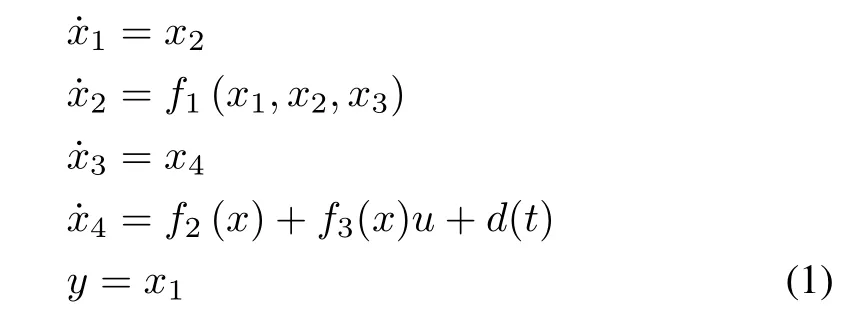
wherex=[x1x2x3x4]T∈R4andy∈R denote the state vector and output respectively.u∈R represents control input;f1(x1,x2,x3),f2(x)andf3(x)are unknown nonlinear smooth functions;d(t)is the external disturbance bounded by a positive constantd0,i.e.,|d(t)|≤d0.Since all physical quantities are in limited region,the statexbelongs to a compact subset Φ∈R4.

De fine the desired trajectory vectoryd,the tracking erroreand an error functionsas

whereci＞0,i=1,2,3 are appropriately chosen such that polynomialλ3+c3λ2+c2λ+c1is Hurwitz,i.e.,e→0 ass→0.The desired trajectory vectoryd∈Φd⊂R4is assumed known and continuous.,,...represent first,second,and third order time derivative ofxd,respectively.The objective is to forcex1to followxd.

From(1),(3)and(4),the time derivative ofscan be written as

where

Assumption 1:The sign off4(x)is known andf4(x)/=0,∀x∈Φ.Without loss of generality,we could assumef4(x)＞0 because of the sign off4(x)being known.

Assumption 2:There is a smooth function(x)such that|f4(x)|≤(x),and(x)is bounded as(x)≤∈R.

III.DESIRED CONTROLLER DESIGN

In order to design the desired controller¯u,we first assume thatf1(x1,x2,x3),f2(x)andf3(x)are known,and the system is ideal and has no disturbance,i.e.,d(t)=0.

Theorem 1:Considering(1),Assumptions 1 and 2,andd(t)=0,the desired controller is designed by

whereεis a positive parameter.Thus,we obtain the result of limt→∞‖e(t)‖=0.

Proof:Settingu=and substituting(6)into(5),we obtain Choosing a Lyapunov function aswe get the time derivative of it as follows:

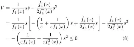
Because off4(x)＞0 and stability theorem,the result≤0 indicates that limt→∞|s|=0,then we have limt→∞‖e(t)‖=0. ¥

According to(8),we come to the conclusion that the convergence rate of the tracking erroreis closely relevant to the parameterε.We change(6)into another form,where the desired controller¯ucan be regarded as a function of the following variable:

and compact subset Φαis de fined as

RBFNNs will be used to design the desired controllerin the following way.Since nonlinear smooth functionsf1(x1,x2,x3),f2(x)andf3(x)are unknown,the ideal controller¯uis not available.The reason whys/εis also chosen in RBFNN as input whensbelongs to it is that it will makesands/εdiffer largely whenεis very small.

whereµεis the RBFNN approximation error such that|µε|≤µ0,µ0＞0,and the radial-basis function vectorh(α)which denotes the output of hidden layer is given by

whereα∈R7is the input vector,and in this study the number of input neural nets in the input layer is seven;mdenotes the number of hidden neural nets in the hidden layer;hjis Gaussian function;Aj=[aj,aj,...,aj]T∈R7;a∈Rmandb∈Rmrepresent the center of the receptive field and the width of Gaussian function respectively.The ideal RBFNN weight vectoris bounded as

To improve the computational procedure,we de fine a positive constant as follows:

IV.ACTUAL CONTROLLER DESIGN

In this section,we propose a single parameter adaptive(SPA)control method.The main contribution is that the number of online adaptive parameters is decreased to only one parameterˆφ,instead of a vectorthus shortening the time on operation.The adaptive controller is designed as follows:

The adaptive law will be given later.Substituting(15)into(5),we have

Adding and subtractingf4(x)(α)on the right-hand side of(16)and from(11),respectively,we obtain

Then,substituting(6)into(17),it yields

Theorem 2:With the controller(15),and the adaptive law

whereγ＞0,κ＞0,the tracking errore(t)in(3)is bounded in the compact subset Φ for all time,and can be made arbitrarily small by using appropriate parameters.The closed-loop system is uniformly ultimately bounded and the statex1will follow the desired trajectoryxd.

Proof:A Lyapunov function could be denoted as

Differentiating(20)with respect to time,and from(18),we have

Using the facts that

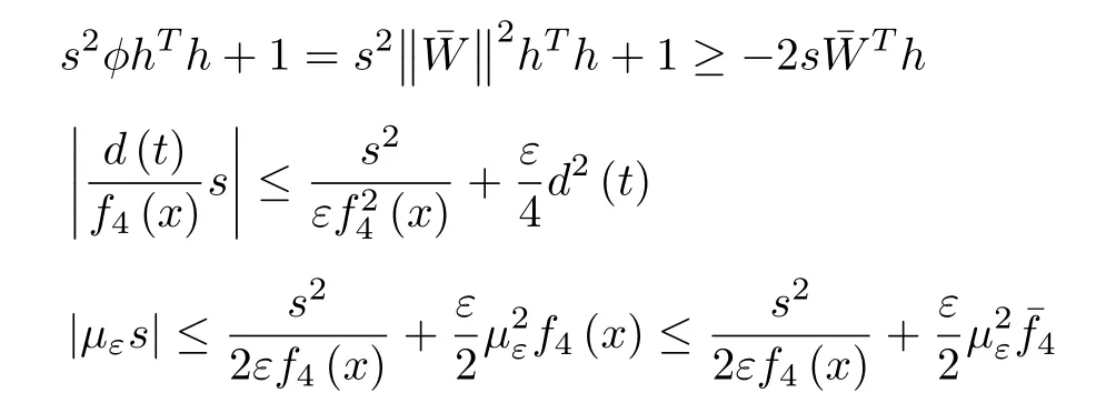
and noting that|µε|≤µ0,|d(t)|≤d0,we obtain

Considering the adaptive law(19),and from(22),we have

Settingκ=η/γ,η＞0,we obtain Solving the above inequality using Lemma B.5 in[24],we have

By the definition ofV,we haveThus,weFrom(23),and notingwe obtain

SinceV(0)is bounded,the inequality(24)shows thatsis bounded asThe inequality(23)also shows thatV(t)is bounded which implies ˜φis bounded too.Thus,the closed-loop system is proven uniformly ultimately bounded.

The inequality(24)indicates that the tracking errore(t)converges to a small residual set Φ for all time,then the statexin system(1)will follow the desired trajectoryxd.The tracking errore(t)can be made arbitrarily small by appropriately choosing the parametersε,ηandγ.The increases inγandη,or decrease inεwill make the tracking performance better.¥

V.SIMULATION RESULTS

In order to prove the effectiveness of the control scheme,we take a CMD system for simulation.Its schematic is shown in Fig.1,and the linearized dynamics in the presence of external disturbance could be written as follows[23]:

whereθ1is the drive angle position;θ2is the load angle position;Jlis the total inertias reflected at the load;Jdis the total inertias reflected at the drive;gr=(rlrpl)/(rp2rd)is the gear ratio;Tdis control torque input;c11is the drive rotary damping(modeled as viscous);c12is the load rotary damping(modeled as viscous);d(t)is the external disturbance,andk=is torsional spring constant.

Fig.1.Schematic of CMD system.

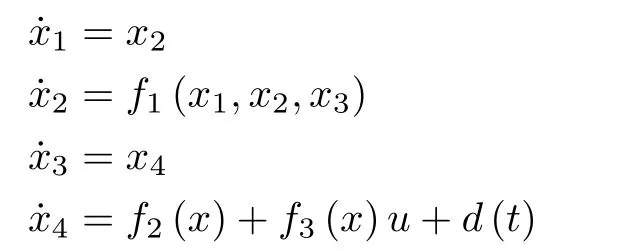
Letx1=θ2andx3=θ1be the state variables,andu=Tdbe the control input,then the dynamics(25)will be changed into the form as follows:

where

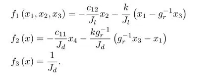
The parameter values in(25)for simulation are given byJd=0.000425kg·m2,Jl=0.3575kg·m2,d(t)=sin(t),c12=0.05(N·m)·s/rad,c11=0.004(N·m·s)/rad,gr=4,k=8.45(N·m)/rad.

The initial states arex(0)=[0.5 0 0 0]T,and the desired signal isxd=sint.The input vector of RBFNN isα=[x1x2x3x4ss/εv]T.The network structure 7-9-1 is used.The parameters ofajandbjin RBFNN must be chosen according to the scope of the input value.If the parameter values are chosen inappropriately,Gaussian function will not be effectively mapped,and RBF network will be invalid.In this example,according to the practical scope ofx1,x2,x3,x4,s,s/εandv,from(10),for each Gaussian function,the parameters ofaandbjare designed asa=0.1×[-2-1.5-1-0.5 0 0.5 1 1.5 2]andbj=5 respectively.The initial weight value is chosen as zero.In the adaptive law(20),the initial condition is(0)=0.The filtered tracking gain parameters in(4)are chosen asc1=27,c2=27,andc3=9.Fig.2 shows the closed-loop RBFNN adaptive control scheme.

The simulations with different design parameters are shown in Figs.3-6 to illustrate the tracking performance of the controller.In Figs.3 and 4,the parameter in the ideal feedback control law(6)is taken asε=0.1 and the adaptation gain constants in the adaptive law(19)are given byη=10 andγ=10.In Figs.5 and 6,the parameters are chosen asε=0.01,η=100 andγ=100.Figs.3-6 show the different tracking errors and control inputs,illustrating the effectiveness of the proposed scheme.By contrast,we validate the conclusion that the smallerεand largerηandγmay improve the tracking performance of the closed-loop system.

Fig.2.Block diagram of RBF control scheme.

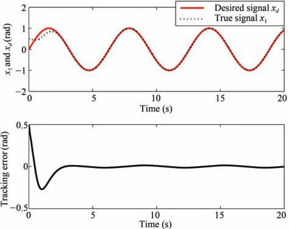
Fig.3. Position tracking performance with the parameters ε =0.1,η =10 and γ=10.

Fig.4. Control input with the parameters ε =0.1,η =10 and γ =10.

VI.CONCLUSION

An adaptive RBFNN control method has been proposed in this paper for a class of SISO nonlinear systems in the presence of bounded disturbances.By designing adaptive controller and adaptive law using a constant parameter,we prove uniform ultimate boundedness of the closed-loop system.Finally,we take the CMD system which satisfies the above mentioned for simulation to con firm the effectiveness of the method.The simulation results show the favorable performance on tracking desired signal and verify the stability of the closed-loop adaptive system through selecting the appropriate parameters.

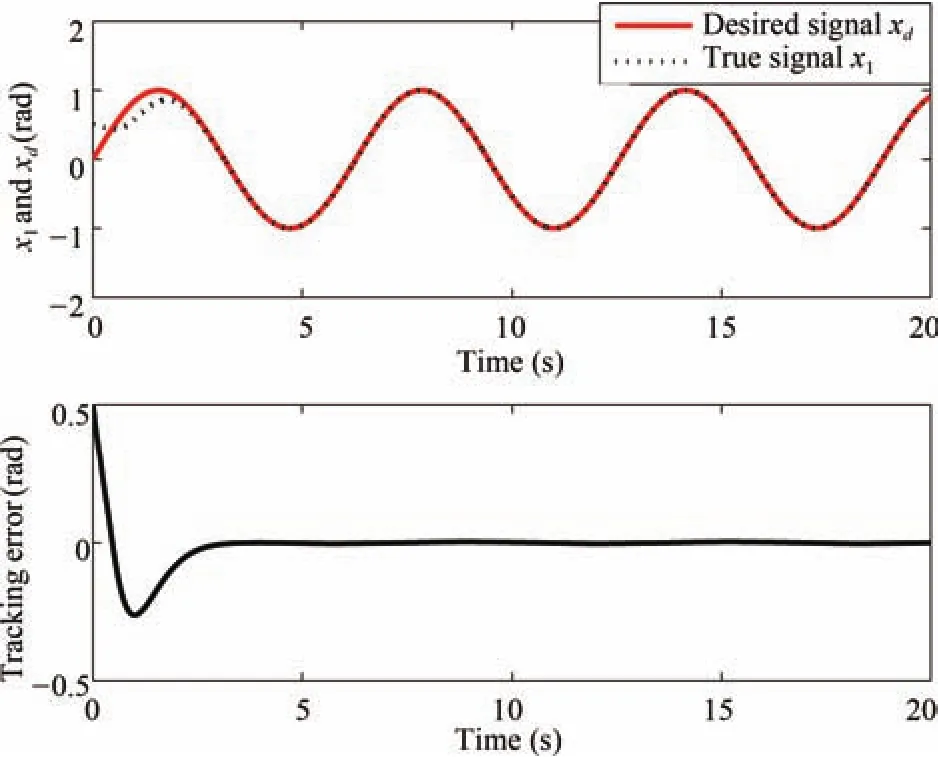
Fig.5.Position tracking performance with the parameters ε=0.01, η =100 and γ=100.

Fig.6.Control input with the parameters ε =0.01,η =100 and γ =100.

[1]M.Hojati and S.Gazor,“Hybrid adaptive fuzzy identification and control of nonlinear systems,”IEEE Trans.Fuzzy Syst.,vol.10,no.2,pp.198-210,Apr.2002.

[2]Y.J.Choi and A.J.Farrell,“Nonlinear adaptive control using networks of piecewise linear approximators,”IEEE Trans.Neural Netw.,vol.11,no.2,pp.390-401,Mar.2000.

[3]S.Ulrich,Z.J.Sasiadek,and I.Barkana,“Modeling and direct adaptive control of a flexible-joint manipulator,”J.Guid.Control Dyn.,vol.35,no.1,pp.25-39,Jan.-Feb.2012.

[4]M.Chen and S.S.Ge,“Direct adaptive neural control for a class of uncertain nonaf fine nonlinear systems based on disturbance observer,”IEEE Trans.Cybern.,vol.43,no.4,pp.1213-1225,Aug.2013.

[5]B.J.Hoagg and D.S.Bernstein,“Retrospective cost model reference adaptive control for nonminimum-phase discrete-time systems,Part 2:Stability analysis,”inProc.2011 American Control Conf.(ACC),San Francisco,CA,USA,2011,pp.2927-2932

[6]A.M.Santillo and S.D.Bernstein,“Adaptive control based on retrospective cost optimization,”J.Guid.Control Dyn.,vol.33,no.2,pp.289-304,Mar.-Apr.2010.

[7]S.Mohan and J.Kim,“Indirect adaptive control of an autonomous underwater vehicle-manipulator system for underwater manipulation tasks,”Ocean Eng.,vol.54,pp.233-243,Nov.2012.

[8]A.Mohammadzadeh,O.Kaynak,and M.Teshnehlab,“Two-mode indirect adaptive control approach for the synchronization of uncertain chaotic systems by the use of a hierarchical interval type-2 fuzzy neural network,”IEEE Trans.Fuzzy Syst.,vol.22,no.5,pp.1301-1312,Oct.2014.

[9]W.He,Y.H.Chen,and Z.Yin,“Adaptive neural network control of an uncertain robot with full-state constraints,”IEEE Trans.Cybern.,vol.46,no.3,pp.620-629,Mar.2016.

[10]W.He,Y.T.Dong,and C.Y.Sun,“Adaptive neural impedance control of a robotic manipulator with input saturation,”IEEE Trans.Syst.Man Cybern.Syst.,vol.46,no.3,pp.334-344,Mar.2016.

[11]W.He,Z.C.Yan,C.Y.Sun,and Y.N.Chen,“Adaptive neural network control of a flapping wing micro aerial vehicle with disturbance observer,”IEEE Trans.Cybern.,vol.47,no.10,pp.3452-3465,Oct.2017.

[12]M.Moradi and H.Malekizade,“Neural network identi fication based multivariable feedback linearization robust control for a two-link manipulator,”J.Intell.Robot.Syst.,vol.72,no.2,pp.167-178,Nov.2013.

[13]V.Goyal,K.V.Deolia,and T.N.Sharma,“Neural network based sliding mode control for uncertain discrete-time nonlinear systems with timevarying delay,”Int.J.Comput.Intell.Res.,vol.12,no.2,pp.125-138,2016.

[14]T.Wang,H.J.Gao,and J.B.Qiu,“A combined adaptive neural network and nonlinear model predictive control for multirate networked industrial process control,”IEEE Trans.Neural Netw.Learn.Syst.,vol.27,no.2,pp.416-425,Feb.2016.

[15]J.Y.Liu,J.Li,S.C.Tong,and C.L.P.Chen,“Neural network controlbased adaptive learning design for nonlinear systems with full-state constraints,”IEEE Trans.Neural Netw.Learn.Syst.,vol.27,no.7,pp.1562-1571,Jul.2016.

[16]D.R.Liu,H.L.Li,and D.Wang,“Neural-network-based zero-sum game for discrete-time nonlinear systems via iterative adaptive dynamic programming algorithm,”Neurocomputing,vol.110,pp.92-100,Jun.2013.

[17]J.K.Liu,Radial Basis Function(RBF)Neural Network Control for Mechanical Systems:Design,Analysis and Matlab Simulation.Berlin,Heidelberg,Germany:Springer,2013.

[18]X.P.Chen,W.X.Shen,M.X.Dai,Z.W.Cao,J.Jin,and A.Kapoor,“Robust adaptive sliding-mode observer using RBF neural network for lithium-ion battery state of charge estimation in electric vehicles,”IEEE Trans.Veh.Technol.,vol.65,no.4,pp.1936-1947,Apr.2016.

[19]R.Yang,V.P.Er,Z.D.Wang,and K.K.Tan,“An RBF neural network approach towards precision motion system with selective sensor fusion,”Neurocomputing,vol.199,pp.31-39,Jul.2016.

[20]S.Li and X.Q.Jiang,“RBF neural network based second-order sliding mode guidance for Mars entry under uncertainties,”Aerosp.Sci.Technol.,vol.43,pp.226-235,Jun.2015.

[21]Y.B.Xing,Y.L.Yu,and K.Z.Zhou,“Composite single neural PID controller based on fuzzy self-tuning gain and RBF network identi fication,”inProc.26th Chinese Control and Decision Conference(2014 CCDC),Changsha,China,2014,pp.606-611

[22]S.S.Ge,C.C.Hang,and T.Zhang,“A direct method for robust adaptive nonlinear control with guaranteed transient performance,”Syst.Control Lett.,vol.37,no.5,pp.275-284,Aug.1999.

[23]O.Kuljaca,N.Swamy,L.F.Lewis,and C.M.Kwan,“Design and implementation of industrial neural network controller using backstepping,”IEEE Trans.Ind.Electron.,vol.50,no.1,pp.193-201,Feb.2003.

[24]M.Krstic,I.Kanellakopoulos,and P.V.Kokotovic,Nonlinear and Adaptive Control Design.New York,USA:Wiley,1995.