An Online Fault Detection Model and Strategies Based on SVM-Grid in Clouds

PeiYun Zhang,,Sheng Shu,and MengChu Zhou,

NOTATIONS

BAC-score Balance accuracy score

CRM Client relation management

ELM Extreme learning machine

LVQ Learning vector quantization

NCZ Not crossing zero

PCA Principal component analysis

RBF Radial basis function

SVM Support vector machine

VM Virtual machines

A1The normal sample set obtained from the first stageB1The abnormal sample set obtained from the first stageCParameterCin an SVM modelDThe set of samples from a cloud systemD′The set of all new samples

The set of all old abnormal samples

DBThe database of samples

MiTheith principal component

PiThe fault probability

RThe cumulative contribution ratio

TA given test set of samples

VThe classified set after fine prediction

Xn×mThe matrix of all attributes

Yn×mThe normalized attribute matrix ofXn×m

aiai∈D′

bjbj∈

b∗The offset of the decision function

cminThe lower bound ofC

cmaxThe upper bound ofC

didi∈D

f(w)Decision function for classification in an SVM

f1The objective function value from a trained SVM

f2The sum ofαifrom a trained SVM

gParametergin an SVM model

gminThe lower bound ofg

gmaxThe upper bound ofg

ljs label

piThe eigenvectors

rjpCorrelation coefficient between standardized attributesjandp

rThe contribution ratio of the principal componentMi

step1 A preset used to increase the value ofC

step2 A preset used to increase the value ofg

vivi∈V

wAn input vector of a samplewjThe vector of a samplej

yijyijis an entry inYn×m

αThe required training errorαiLagrange multiplier

The solution to(1)µThe threshold in parameter optimization

Θ The threshold for fine fault predictionγThe threshold for updating cloud faultsλLearning rate

I.INTRODUCTION

THE past decade has witnessed the rapid development and wide applications of cloud computing technology.Many large IT companies have launched their own cloud platforms,such as Google,Alibaba and Amazon cloud.Open source technologies have gained much development for cloud computing,including Eucalyptus and Open Stack.Currently,e-commerce,social networks[1]and other Internet services[2]have become inseparable parts of people’s daily work and life.Many applications are deployed on cloud platforms,such as sale force client relation management(CRM).Many researchers are devoted to cloud scheduling[3]-[5],and resource allocation[6]so as to improve the quality of cloud services[7]-[9].However,the complexity and diversity of cloud applications and environment bring about cloud faults from time to time,which affect the quality of services.The faults not only have a huge bad impact on people’s normal life and work,but also cause serious economic losses in business.For example,the Amazon crash happened in August 2013 in less than an hour,resulted in about$5 million loss,and badly affected numerous customers.Efficient monitoring and accurate detection of cloud faults are prerequisites for stable operations of cloud services.

Faults in distributed systems are generally caused by hardware faults and software failures.For example,software bugs related to deadlocks,concurrency and other complex relations account for 15%-80%[10]of all software failures detected after release[11],[12].These kinds of failures are randomly produced and are difficult to be reproduced.These software failures are hard to be detected in software development and testing phases.It is also difficult for system managers to manually track their statuses at run time.Although virtualiza-tion provides software failure isolation among different virtual machines(VM),the virtualization infrastructure including the hypervisor and privileged VMs remains vulnerable to hardware errors[13].Hence,it is necessary for service providers to adopt fault detection technologies in clouds,such as commonly used online detection systems,which can predict cloud faults before their happening and thus reduce the corresponding loss.Tellme Networks discusses the time of fault recovery in distributed systems.It shows that often 75%of time is used to detect faults,and 18%of time is required to diagnose faults[14].Advanced fault detection strategies can be used to avoid about 65%of faults in clouds[15].Therefore,efficient and accurate detection of cloud faults can help ensure stable operations and reliable services for cloud systems.There are some online detection systems.However they face some problems,such as low accuracy.

Traditional fault detection methods can detect faults when the monitored running status deviates from the set values[11].However,existing solutions are hard to detect faults in a large-scale dynamic distributed cloud computing environment because of the following reasons[16]:

1)Elastic and on-demand services based on VMs in the clouds produce many new issues,such as VM re-sizing,migration,and cloning in a dynamic cloud context.The dynamic cloud environment makes applications change from time to time with workloads and resource allocation.

2)Applications deployed in a large scale data center with nodes make fault detection systems collect a large number of sample attribute values from many layers,e.g.,network and hardware.

3)Because services are usually transparent to system operators,it is infeasible to use traditional methods to analyze a service’s architecture,e.g.,dependencies and interactions among components.It is also difficult to detect faults without domain knowledge.

Hence,new detection approaches for detecting faults are highly demanded.We propose an online detection model and strategies based on SVM-Grid for predicting emerging problems in clouds.The proposed model mainly predicts faults with the collected samples from the running status of cloud systems.Some strategies are utilized to improve the detection performance of the model.

The rest of the paper is organized as follows:Section II gives a brief literature review.Section III introduces the proposed model and gives its analysis.Section IV gives the experimental results and their analysis.Section V makes some conclusions and indicates the future work.

II.RELATED WORK

Many researchers have been devoted to the field of fault detection.Fault detection models can be mainly divided into two classes:rule and statistics-based ones.

A.Rule-based Detection Models

Rule-based detection models discern a faultbased on its characteristics.Fault databases are constructed based on prior descriptions.When attributes of samples are matched with a fault’s features in fault sample database,we claim that the samples are fault ones.Their representative methods include:

1)Signature method:It de fines fault characteristics as signature.Are finet al.[17]propose a framework named Flow Diff to model the behavior of a data center by using infrastructure,application,and task signatures.The infrastructure signature captures the physical topology of a network,the mapping of applications to servers,and baseline performance parameters(such as link utilization and end-to-end delay);application one captures the behavior of each application(e.g.,response time distribution and flow statistics)and how applications interact with each other;while task one models the valid behavioral changes performed by the operator or applications(e.g.,VM migration).

2)Similarity judgment:It sets up a fault sample database according to historical knowledge that includes fault characteristics,faults occurrences and how to fix faults.Chenet al.[18]present an instance-based approach to diagnose failures by storing historical faults in a database and retrieving similar instances in the occurrence of faults.

3)Decision tree:It can judge whether faults happen or not based on mappings between object attributes and object values.Kicimanet al.[19]propose a methodology by using a decision tree for automated fault detection in Internet services,which includes observing low-level internal structural behaviors of services,modeling majority of system behaviors as correct ones,and detecting anomalies in these behaviors as possible symptoms of faults.Linet al.[20]present an efficient adaptive failure detection mechanism based on Volterra series that uses a Volterra filter for time series prediction and a decision tree for decision making.

B.Statistics-based Detection Models

Statistics-based detection models construct fault detection models based on the data collected from the cloud systems.Important methods include:

1)Neural networks[21]-[26].Liuet al.[21]propose a prediction model based on an optimized neural network with a multilevel genetic algorithm.Liet al.[22]describe a fault diagnosis model based on a neural network,and establish relations between network fault information and fault pattern output.Yanet al.[23]adopt a neural network model to predict faults in electric power communication systems.Tamuraet al.[24]use it to detect software faults in a cloud environment.A neural network-based method is applied to intelligently classify inverter switch faults[25].

2)Improved learning vector quantization(LVQ)based on back propagation(BP)neural networks[27]-[30].Maliket al.[27]present an LVQ neural network for classification problems.Liet al.[28]use it for fault classification for analog circuits.Liuet al.[29]utilize it to classify samples into normal samples and faults.Bassiunyet al.[30]combine empirical mode decomposition and LVQ to detect faults.

3)Support vector machine(SVM)[31]-[38].Leeet al.[34]propose a detection model based on SVM to find opens witch faults.SVM can be used to address two-class(normal or abnormal)and multi-class problems[37].Zhanget al.[38]propose a method for predicting the types of weather via multiclass SVM based on the photovoltaic(PV)power data and partial meteorological data.

Both rule and statistics-based detection models have encountered their own challenges.The first one requires too much information about the internal systems and the efficiency of its online analysis is low.For the second one,neural network-based methods require a large number of training samples.In reality,it is extremely difficult to collect a sufficient number of abnormal samples.

In contrast with the first one,in recent years,the second one has attracted more researchers’attention because of its following advantages:

1)Neither historical knowledge,nor prior descriptions of fault characteristics of cloud systems are required.statistics-based detection models use the ports to monitor and collect the running data of cloud systems without deeply knowing the internal structure of cloud systems.Hence,it has a wide application scope.

2)The corresponding characteristics of cloud systems can be detected efficiently and accurately through online monitoring of cloud systems and timely analysis of collected data.

As one of the popular statistics-based detection models,Rahulamathavanet al.[37]point out that SVM has strong mathematical foundations and high reliability in many practical applications.However,traditional SVM models suffer from high time cost.Such high cost is caused by a)lack of optimization of SVM parameters and b)lack of timely updating of the sample space,which also result in low accuracy.Hence,a new model is highly demanded to address these two issues.

We propose an online fault detection model based on SVMGrid,which targets at solving the above problems,including improving the accuracy of detection and efficiency of traditional SVM models.The proposed model makes the following improvements:

1)It uses a Grid method to optimize the parameters of an SVM model to achieve fine-tuned prediction for higher accuracy;

2)It uses a two-stage strategy for preliminary fault prediction and fine prediction for cloud faults;and

3)It utilizes a novel strategy for updating the fault sample database so as to further reduce the computational time of fault detection.

Next,we present and analyze the proposed method.

III.CLOUD FAULT DETECTION MODEL BASED ONSVM-GRID

The proposed model based on SVM-Grid is constructed as follows:

1)A fault detection model is set up based on SVM.The Grid method is based on[25].We use it to optimize two important parameters for the model and

2)Strategies for predicting cloud faults and updating fault sample database are proposed and used to optimize the model and improve its performance.

A.Fault Prediction Model

Some definitions related to the proposed model are given before its introduction.

Normal samples are those collected when the cloud systems run normally.Abnormal ones are those collected when they run wrongly.

We treat cloud fault detection as a binary classification problem.LetSbe a given cloud sample training set.

wherewj∈Rnis the vector of a samplej,j∈{1,2,...,m}andljis its label.

Based on SVM[44],we can transform a cloud fault detection problem into the following second-order constrained programming problem:

wherei,j∈{1,2,...,m},αiandαjare the Lagrange multipliers.K(wi,wj)is the kernel function.ParameterCdenotes the penalty dealing with constraint violation for the model.The cloud fault detection problem is further translated into finding the optimal hyperplane problem.Its decision function is as follows:wherewis an input vector of a sample,a∗iis the solution to(1)andb∗is the offset.

When constructing a fault detection model based on SVM,we first need to select an appropriate kernel function.The commonly used ones include a linear kernel function,polynomial kernel function and radial basis function(RBF).RBF can approximate any nonlinear function.It has good generalization ability with fast convergence.It also has fewer parameters to be determined.It can reduce a model’s complexity and improve efficient prediction for faults.Hence,we adopt RBF as the kernel function of the proposed fault detection model.

There are two key parametersCandgof SVM in the proposed model to be optimized.Motivated by[39],we use the Grid method to do so as shown in Algorithm 1.

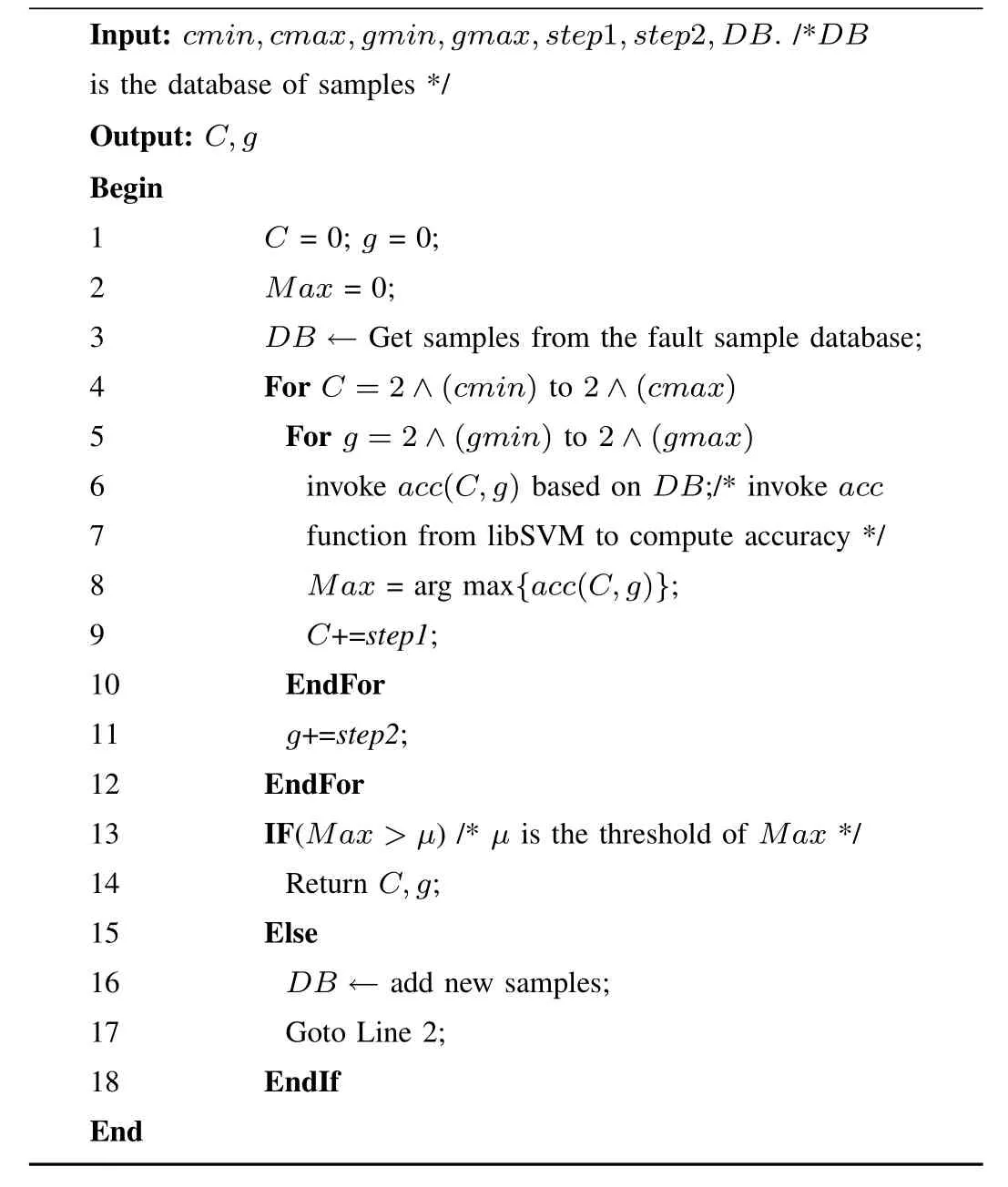
Algorithm 1.Parameter Optimization

Algorithm 1 aims to find the best values for parametersCandgin a hyper plane.The ranges of parametersCandgare derived from(2-10,210).In Lines 9 and 11,step1 andstep2 are two preset values that are used to increase the values of C SPACE needed before ”and”andgrespectively.We setcmin=gmin=2-10andcmax=gmax=210.If the accuracy of the trained model cannot satisfy the requirement,we need to add additional samples from the existing dataset to re-train it until the requirement is satisfied.If there are no more additional samples for retraining,we have to decrease the accuracy requirement,i.e.,decreasing the threshold in Algorithm 1.

Based on the proposed model with optimized parametersCandg,the normal and abnormal samples for training are used to train the model.After training,a hyperplane is obtained.

We add two strategies to the obtained model to improve its performance,i.e.,fault prediction strategy and fault updating one.

B.Fault Prediction Strategy

The cloud fault prediction strategy has two stages.

1)Preliminary fault prediction

At the first stage,we use the hyperplane of the trained SVM model to divide samples into two classes:normal and abnormal samples,i.e.,setA1with normal samples andB1with abnormal ones.We predict the fault probability based on the distance from abnormal samples to the SVM hyperplane.The bigger the distance,the greater fault probability.Because of SVM’s inaccuracy,some abnormal samples may be misclassified as normal ones.LetTbe a given testing set of samples.

The preliminary fault prediction is realized in Algorithm 2.

Algorithm 2.Preliminary Fault Prediction

Algorithm 2 gives a preliminary fault prediction.For abnormal samples near the hyperplane,they may sway much and have a greater likelihood to be misclassified as normal ones.If they are used for fault prediction,they may lead to low accuracy.Hence,we use the second stage prediction strategy to improve the prediction accuracy.

2)Fine prediction for cloud faults

The first stage has preliminarily classified all samples into normal and abnormal ones.We have to deal with those abnormal samples(near the hyperplane)that are misclassified as normal ones.After the hyperplane is obtained,the fault probabilityPifor sampleito be a fault is as follows:

wherevi∈Vis the decision value of sampleifrom the first stage classification.viis negative if sampleiis abnormal;otherwise positive.vican be zero in theory(i.e.,an undecided sample),but we have not obtained any zero results in our experiments.Note thatV,f1andf2come from the output of Algorithm 2.The process of fine-tuned fault prediction is proposed in Algorithm 3.

In Algorithm 3,Θ∈(0,1)is the threshold of the fault probability of samples.WhenP[i]≤Θ,we regard sampleias an abnormal one.We useB2to denote the set of the abnormal samples obtained from the second stage.

Algorithm 3.Fine Fault Prediction

Letwibe the vector of abnormal samplei.After two stages of fault prediction based on Algorithms 2 and 3,wisat is fies:

C.Fault Updating Strategy

Because the cloud faults increase gradually,we need to add them into the fault sample database.We need to consider reducing extra time for the clouds when new abnormal samples are added.To avoid adding the same or more similar samples to the abnormal sample database,we need to compute the similarity between a new abnormal sample and an old one as follows:

whereaiandbjare two vectors representing new abnormal sampleiand old abnormal samplej,respectively.ai·bjis an inner product of vectorsaiandbj.The fault updating process is given in Algorithm 4.

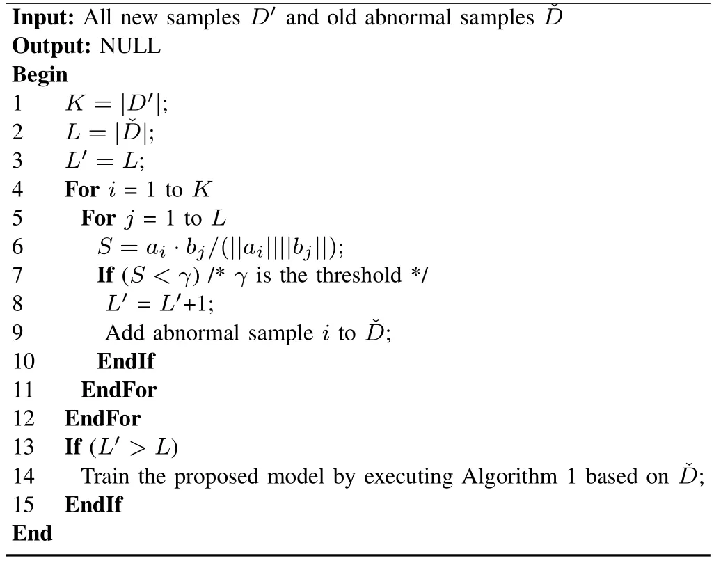
Algorithm 4.Updating Cloud Faults

In Algorithm 4,KandLrepresent the total number of old and new fault samples,respectively.ai∈D′,1≤i≤Kandbj∈ˇD,1≤j≤L.The similaritySbetweenaiandbjis computed based on a cosine vector.If their similarity is high enough,the new fault sampleiis regarded as being a similar fault,and should not be added into the database.Otherwise,sampleiis added into it.The proposed model is then trained based on the updated fault sample database.Algorithm 4 can avoid updating for each new abnormal sample,but for only new abnormal samples with enough difference from all the prior ones.Therefore,it decreases computing burden.

IV.E XPERIMENTS

A.Experimental Environment

In this work,simulation experiments are conducted based on publicly available data from Google2 application cluster of Google Corporation.The total size of this dataset is about 40GB.It contains more than 12500 virtual machines running during 29days.Data items New line.are acquired every 300 seconds.The dataset is available at http://github.com/google/cluster-data

500 normal samples and 500 abnormal samples are selected randomly from the dataset.In order to validate the capability of the model,the dataset is divided into 5 groups.4 copies are used for training the proposed model,and the remaining one is used for model prediction.The average values are computed.We execute 10 trials in experiments and compute the average values based on 5 groups of data.

Experimental environment includes MATLAB 2017,Intel Core i5,2.3GHz and 4G memory and libSVM-3.1[37],[39].Thresholds:µ=85%in Algorithm 1,Θ=0.5 in Algorithm 3 andγ=0.8 in Algorithm 4.

B.Attribute Optimization

If all attributes of samples collected from a cloud environment were used by the fault detection model,the computational overhead would be too large.Therefore it is necessary to make a reasonable choice for attributes while meeting a model’s accuracy requirements.The monitored attributes of a cloud system usually have certain correlation.We use the Pearson correlation coefficient to analyze linear correlation among attributes.Based on principal component analysis(PCA)[40],a new attribute is constructed based on the linear combination of attributes.It should represent as many original attributes as possible in disparate conditions.In the end,several attributes are synthesized to represent most if not all of attributes based on the linear correlation of the latter.

LetDbe the set of samples from a cloud system as follows.

wherenis the cardinality of setDanddi∈D.

wherexijrepresents thejth attribute of sampledi.

Taking a Google dataset for example,we have the following 10 attributes:

mean CPU usage rate

canonical memory usage

assigned memory usage

unmapped page cache memory usage

total page cache memory usage

maximum memory usage

mean disk I/O time

mean local disk space used

maximum CPU usage

maximum disk I/O time.

Because of different dimensions and different classes of numerical values of attributes,we should normalize all the original attributes.We then calculate the Pearson correlation coefficient among attributes.We finally reduce the number of attributes for model training via PCA so as to reduce the computational overhead while ensuring the model accuracy.

The process of attribute optimization is as follows.

1)Normalize attributes

There arencollected samples,each of which hasmattributes.LetXn×mbe the matrix of all non-negative attributes:

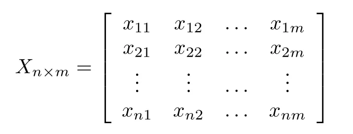
The normalized attribute matrix ofXn×misYn×mwhose entry at(i,j),i∈{1,2,...,n}andj∈{1,2,...,m},is:

After(6),the sum of all components in a column is one.

2)Calculate Pearson correlation coefficient

The closer the correlation coefficient is to 1 or-1,the stronger the correlation is.The closer the correlation coefficient is to 0,the weaker the correlation is.Generally,the threshold is set as 0.8,requiring that,two attributes are very strongly correlated.

a)Calculate the correlation coefficientrjpbetween standardized attributesjandp

where

j,p∈{1,2,...,m}.

b)Construct the removal matrixG

We use Gaussian elimination to makeGas.For example:

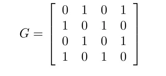
During Gaussian_elimination,swapping two rows is not permitted because each row has its own meaning.After Gaussian_elimination forG,we obtain as follows:

De fine:

where

andi∈{1,2,...,n}andqis a column vector,q(i)∈q.We shrinkYn×mby removing columniin it ifq(i)=0.For example,given:

we have

For our samples,after calculating the Pearson correlation coefficient for 10 attributes,we remove two very strongly correlated attributes,i.e.,canonical memory usage and assigned memory usage.Hence,eight attributes are obtained.

c)Select attributes with PCA

To reduce systems’overhead,we reduce the number of attributes involved in the model calculation.A new attribute is constructed such that it covers the information of original attributes as much as possible.

Using PCA to calculateZis as follows:

LetCbe the correlation coefficient matrix ofZ.C=ZTZ/(n-1).Letλ1≥λ2≥···≥λn＞0[41]be eigen values ofCandi∈{1,2,...,n}.Letpibe eigen vectors.Miis theith principal component ofZ,andMi=piZ.The contribution ratiorof the principal componentMiis as follows:

LetRbe the cumulative contribution ratio of principal components as follows:

M≤nis the number of attributes inZ.N≤Mdenotes the number of principal components when cumulative contribution ratioRis not less than the given threshold.The number of principal components is decided byR.Generally,R≥95%.The ratios of principal components are shown in Fig.1.

Fig.1.The ratios of principal components.

As shown in Fig.1,after the correlation analysis through the Pearson correlation coefficient for 10 attributes,5 principal components are obtained,which contain 95%of information in 10 attributes via PCA.They clearly keep the vast majority of 10 attributes information while reducing the number of attributes by half.Hence,it can reduce the complexity of the proposed model.Three rows of values of the five principal components are shown in Table I.

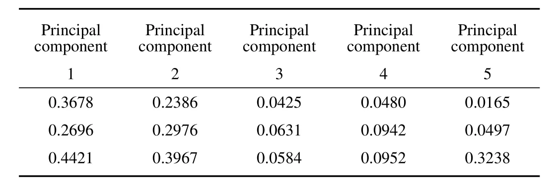
TABLE ISOME VALUES OF THE FIVE PRINCIPAL COMPONENTS

C.Parameter Optimization

To train a better model,we need to optimize the model’s key parametersCandgof SVM.Experimental results are shown in Figs.2 and 3.

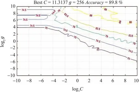
Fig.2. The optimized parameters of RBF(contour plot).

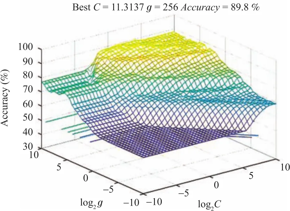
Fig.3. The optimized parameters of RBF.

Different values of parametersCandghave different effect on accuracy of the proposed trained model.As shown in Figs.2 and 3,the initial range of bothCandgis(2-10,210).Here,we use log2Cand log2gto deal with the range of values.Values ofcmaxandgmaxboth are 210.In Fig.2,a contour line shows the same accuracy with different co-ordinates.The higher parameterC,the lower accuracy of the model.Hence,when reaching the same accuracy,we select smallerCat the higher contour line.We obtain the bestC=11.3137 andg=256 through the grid method of Algorithm 1.The accuracy of the trained model is 89.8%.From Fig.3 we can clearly see that the accuracy reaches about 90%.

D.Comparing the Proposed Model With BP and LVQ

We compare the proposed model with BP[24]and LVQ[27]models.

A BP model[24]is a kind of multi layer feed-forward neural network according to the error back-propagation training.Its basic idea is to use the gradient descent method and gradient search technology.Its goal is to reach the minimum mean square error between actual output and predicted outputs.Maximum training count is 1000.Learning rateλ=0.1.The required training errorα=0.1.After testing two situations:α=0.1 andα=0.01,we find that the result is better atα=0.1.Smallerαinduces a higher misclassification rate,i.e.,the accuracy of the classification is lower.The other values of parameters of BP are by default as shown in MATLAB 2017.

An LVQ model[27]is a kind of a feed-forward network in which a supervised learning method is used to train its competitive layer.The sameαandλare used as those in the proposed and BP models.

For sample prediction,it produces four kinds of results:

1)Normal samples are predicted as normal ones.LetNNbe the number of such samples.

2)Normal samples are predicted as abnormal ones.LetNFbe the number of such samples.

3)Abnormal samples are predicted as normal ones.LetFNbe the number of such samples.

4)Abnormal samples are predicted as abnormal ones.LetFFbe the number of such samples.

Because accuracy is very important for fault prediction for the three models,we use it to evaluate them.

The results of accuracy are shown in Fig.4.

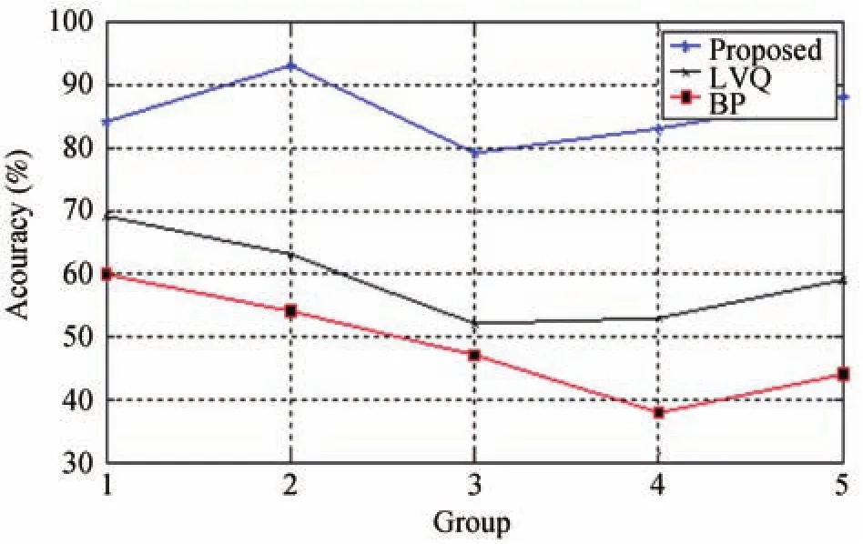
Fig.4. Accuracy of three models.

As shown in Fig.4,in order to avoid random effects on the results,the three models have significant differences in accuracy via 5 sets of experiments.We can see that BP has higher accuracy than LVQ while the proposed model well outperforms BP and LVQ.We also test the time cost of the three models as shown in Fig.5.

From Fig.5 we can see that LVQ has the highest training time cost.BP is much faster than LVQ while the proposed model is the fastest.

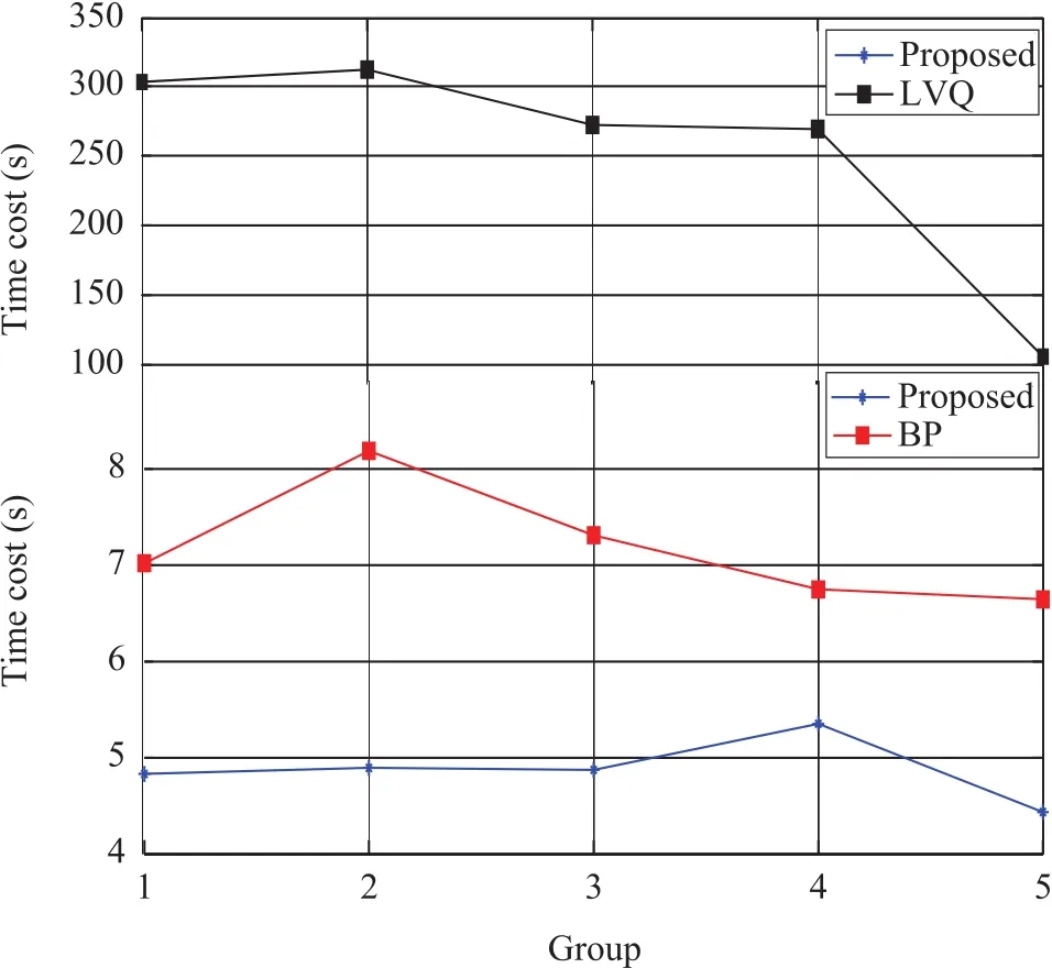
Fig.5. Training time of the proposed,LVQ and BP.

E.Proposed Model vs.Traditional SVM

Traditional models based on SVM[37]simply classify samples via the SVM hyperplane as shown in[31]-[38].It lacks parameter optimization and fine prediction.In view of practical application problems,strategies of the fine prediction and updating fault sample databases are adopted in the proposed model,so as to increase the accuracy and reduce training time.

The SVM classification involves two phases:training and testing phase.In the first phase,SVM is trained by using labeled data belonging to different classes.In the second phase,unlabeled data samples can be classified and labeled to the matched classes through the trained SVM model.

We use Precision,Recall,F-score and BAC-score to make a comprehensive comparison between the proposed one and traditional SVM model.

whereSendenotes the sensitivity degree andSpedenotes the specificity of fault detection,which are computed as

and

The experimental results are shown in Figs.6-10.

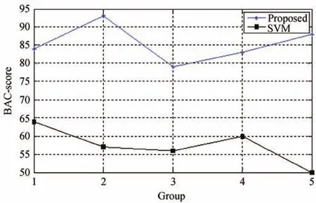
Fig.6. Accuracy of the proposed method and a traditional SVM.

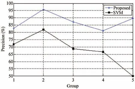
Fig.7. Precision of the proposed method and a traditional SVM.

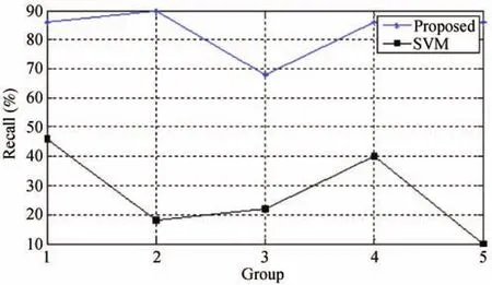
Fig.8. Recall of the proposed method and a traditional SVM.

Fig.9. F-score of the proposed method and a traditional SVM.

Fig.10. BAC-score of the proposed method and a traditional SVM.

From Figs.6-10 we conclude that the accuracy,precision,recall,F-score and BAC-score of the proposed model are better than SVM’s,especially for groups 2 and 5.Because the time cost of the two models exhibits insignificant difference,we do not illustrate them in this paper.

F.Proposed Model vs.State-of-the-art Model

We compare the prediction performance between the proposed method and a neural network-based method called extreme learning machine(ELM)[42].Note that the ELM’s parameter setting and training follow[42].We execute the same experiment based on five groups of testing data as the previous ones.

In Table II,there are five functions for ELM,which are sig,sin,hardlim,tribas and radbas.The number of hidden neurons is 20,40,60,80 and 100,respectively.By taking function sig and 20 hidden neurons as an example,the accuracy values of five groups are 0.72,0.54,0.48,0.55 and 0.67,respectively.From the former experimental results in Figs.4 and 6,we can see that the average values of five groups of the proposed method are higher than the results from ELM in Table II.

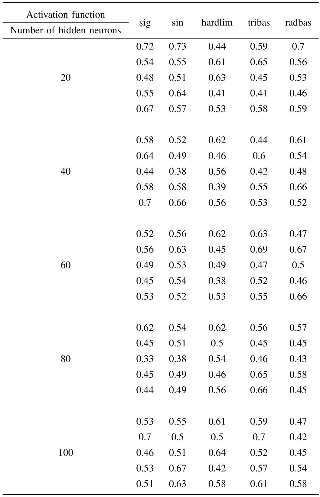
TABLE IITHE ACCURACY RESULTS BYUSING ELM

G.Statistical Test

We perform the statistical test for the proposed method and the other prior methods.We execute the same experiment based on 5 groups of testing data as the previous ones by using SPSS[43],which is commercially available and widely-used software for data analysis.

From Table III,we can see that the proposed method well outperforms ELM in accuracy.By using the proposed method and ELM,F-value=1.50.We obtainp-value ofF-test=0.26,which is bigger than the significance level 0.05.Thus the assumption of equal variance is accepted.Then,we obtainp-value ofT-test=5.17E-4 based on the equal variance result.Because it is smaller than significance level 0.05,the assumption of equal means is rejected.In other words,the proposed method and ELM have statistically significant difference between their average accuracy results.In addition,the 95%confidence interval of mean difference of samples does not cross 0.From their mean accuracy at 85.4(the proposed method’s)and 60(ELM’s),it is easy to conclude that the proposed method is much better than ELM.We can draw the similar conclusion that the proposed method outperforms BP and LVQ.

From Table IV,we can see that the proposed method well outperforms SVM inF-score.We haveF-value at 5.56 andp-value ofF-test at 0.046.Sincep-value is smaller than the significance level 0.05,they have statistically significant difference between their variances inF-score results.We obtainp-value ofT-test=0.001 based on unequal variance result.Because 0.001 is smaller than significance level 0.05,thus the assumption of equal means is rejected.We can conclude that the proposed method and SVM have statistically significant difference between their average values inF-score.In addition,the 95%confidence interval of mean difference of samples does not cross 0.From the proposed method,the average values are 84.95 and from SVM it is 37.12,we conclude that the proposed method is much better than SVM.The experimental results in accuracy,precision,recall and BAC-score from these methods also lead to the same conclusion that the proposed method well outperforms its peers.From the analysis of results obtained via ELM and SVM,we conclude that ELM is better than SVM.

TABLE IIISTATISTICAL TEST FOR THE PROPOSED METHOD VS.BP,LVQ AND ELM IN MEAN ACCURACY(NCZ=NOT CROSSING ZERO)

TABLE IVSOME STATISTICAL TESTS OF THE PROPOSED METHOD VS.SVM INACCURACY,PRECISION,RECALL,F-SCORE ANDBAC-SCORE

V.CONCLUSIONS

Online fault detection is very important for cloud stability.Many detection models need to know too much about the internal cloud systems.The most adopted models based on traditional SVM suffer from the problems of low accuracy.To address them,the work proposes a new online fault detection model based on SVM-Grid.The model is constructed based on SVM and its key parameters are optimized by the grid method.To further improve prediction performance and decrease time cost,the methods for fine-tuned prediction and updating fault sample databases are proposed.

We compare the proposed model with BP and LVQ.The experimental results with a Google dataset clearly show that the proposed model has better accuracy and lower time cost than its two peers.We also compare the proposed model with the traditional SVM model(without using attribute optimization,fine-tuned prediction and database update).The experimental results show that the proposed model achieves better accuracy,precision,recall,F-score and BAC-score than the latter.The experimental results also show that the proposed method is better than ELM.

This work can predict the occurrence of faults in clouds;however it is difficult to locate the reasons that cause faults.This is to be addressed as our the future work.The method can also be modified to predicate faults in other environments,such as Internet of Things[45]-[49].

[1]M.M.Hassan,M.Abdullah Al-Wadud,and G.Fortino,“A socially optimal resource and revenue sharing mechanism in cloud federations,”inProc.19th IEEE Int.Conf.Computer Supported Cooperative Work in Design,Calabria,Italy,2015,pp.620-625.

[2]G.Fortino,A.Guerrieri,W.Russo,and C.Savaglio,“Integration of agent-based and cloud computing for the smart objects-oriented IoT,”inProc.18th IEEE Int.Conf.Computer Supported Cooperative Work in Design,Hsinchu,Taiwan,China,2014,pp.493-498.

[3]H.T.Yuan,J.Bi,W.Tan,M.C.Zhou,B.H.Li,and J.Q.Li,“TTSA:An effective scheduling approach for delay bounded tasks in hybrid clouds,”IEEE Trans.Cybern.,vol.47,no.11,pp.3658-3668,Nov.2017.

[4]H.T.Yuan,J.Bi,W.Tan,and B.H.Li,“CAWSAC:Cost-aware workload scheduling and admission control for distributed cloud data centers,”IEEE Trans.Automat.Sci.Eng.,vol.13,no.2,pp.976-985,Apr.2016.

[5]P.Y.Zhang and M.C.Zhou,“Dynamic cloud task scheduling based on a two-stage strategy,”IEEE Trans.Automat.Sci.Eng.,2017.doi:10.1109/TASE.2017.2693688.

[6]J.Bi,H.T.Yuan,W.Tan,M.C.Zhou,Y.S.Fan,J.Zhang,and J.Q.Li,“Application-aware dynamic fine-grained resource provisioning in a virtualized cloud data center,”IEEE Trans.Automat.Sci.Eng.,vol.14,no.2,pp.1172-1183,Apr.2017.

[7]Y.N.Xia,M.C.Zhou,X.Luo,Q.S.Zhu,J.Li,and Y.Huang,“Stochastic modeling and quality evaluation of infrastructure-as-aservice clouds,”IEEE Trans.Automat.Sci.Eng,vol.12,no.1,pp.162-170,Jan.2015.

[8]W.B.Zheng,M.C.Zhou,L.Wu,Y.N.Xia,X.Luo,S.C.Pang,Q.S.Zhu,and Y.Q.Wu,“Percentile performance estimation of unreliable IaaS clouds and their cost-optimal capacity decision,”IEEE Access,vol.5,pp.2808-2818,Feb.2017.

[9]M.H.Ghahramani,M.C.Zhou,and C.T.Hon,“Toward cloud computing QoS architecture:Analysis of cloud systems and cloud services,”IEEE/CAA J.Autom.Sinica,vol.4,no.1,pp.6-18,Jan.2017.

[10]K.Trivedi,G.Ciardo,B.Dasarathy,M.Grottke,A.Rindos,and B.Varshaw,“Achieving and assuring high availability,”inProc.IEEE Int.Symp.Parallel and Distributed Processing,Miami,FL,USA,2008,pp.1-7.

[11]G.F.Jiang,H.F.Chen,and K.Yoshihira,“Modeling and tracking of transaction flow dynamics for fault detection in complex systems,”IEEE Trans.Dependable Secure Comput.,vol.3,no.4,pp.312-326,Oct.-Dec.2006.

[12]M.Jiang,M.A.Munawar,T.Reidemeister,and P.A.S.Ward,“Efficient fault detection and diagnosis in complex software systems with information-theoretic monitoring,”IEEE Trans.Dependable Secure Comput.,vol.8,no.4,pp.510-522,Jul.-Aug.2011.

[13]X.Xu and H.H.Huang,“On soft error reliability of virtualization infrastructure,”IEEE Trans.Comput.,vol.65,no.12,pp.3727-3739,Dec.2016.

[14]M.Y.Chen,A.Accardi,E.Kiciman,J.Lloyd,D.Patterson,A.Fox,and E.Brewer, “Path-based faliure and evolution management,”inProc.1st Symp.on Networked Systems Design and Implementation,San Francisco,California,USA,2004,pp.309-322.

[15]D.Oppenheimer,A.Ganapathi,and D.A.Patterson,“Why do internet services fail,and what can be done about it?,”inProc.4th Conf.USENIX Symp.Internet Technologies and Systems,Seattle,Washington,USA,2003,pp.165-171.

[16]T.Wang,W.B.Zhang,C.Y.Ye,J.Wei,H.Zhong,and T.Huang,“FD4C:Automatic fault diagnosis framework for web applications in cloud computing,”IEEE Trans.Syst.Man Cybern.Syst.,vol.46,no.1,pp.61-75,Jan.2016.

[17]A.Are fin,V.K.Singh,G.F.Jiang,Y.P.Zhang,and C.Lumezanu,“Diagnosing data center behavior flow by flow,”inProc.33rd Int.Conf.Distributed Computing Systems,Philadelphia,PA,USA,2013,pp.11-20.

[18]H.F.Chen,G.F.Jiang,K.Yoshihira,and A.Saxena,“Invariants based

failure diagnosis in distributed computing systems,”inProc.29th Symp.Reliable Distributed Systems,New Delhi,India,2010,pp.160-166.

[19]E.Kiciman and A.Fox,“Detecting application-level failures in component-based Internet services,”IEEE Trans.Neural Netw.,vol.16,no.5,pp.1027-1041,Sep.2005.

[20]R.H.Lin,B.D.Wu,F.C.Yang,Y.Zhao,and J.X.Zhou,“An efficient adaptive failure detection mechanism for cloud platform based on volterra series,”China Commun.,vol.11,no.4,pp.1-12,Apr.2014.

[21]Q.Liu,F.Zhang,M.Liu,and W.M.Shen,“A fault prediction method based on modified Genetic Algorithm using BP neural network algorithm,”inProc.IEEE Int.Conf.Systems,Man,and Cybernetics(SMC),Budapest,Hungary,2016,pp.4614-4619.

[22]C.L.Li,X.S.Zong,and Gudake,“A survey of online fault diagnosis for PV module based on BP neural network,”inProc.Int.Conf.Smart City and Systems Engineering(ICSCSE),Zhangjiajie,Hunan,China,2016,pp.483-486.

[23]S.Yan,Y.J.Liu,and F.J.Guan,“The application of BP neural network algorithm in optical fiber fault diagnosis,”inProc.14th Int.Symp.Distributed Computing and Applications for Business Engineering and Science,Guiyang,China,2015,pp.509-512.

[24]Y.Tamura,Y.Nobukawa,and S.Yamada,“A method of reliability assessment based on neural network and fault data clustering for cloud with big data,”inProc.2nd Int.Conf.Information Science and Security,Seoul,South Korea,2015,pp.1-4.

[25]Z.J.Huang,Z.S.Wang,and H.G.Zhang,“Multilevel feature moving average ratio method for fault diagnosis of the microgrid inverter switch,”IEEE/CAA J.Autom.Sinica,vol.4,no.2,pp.177-185,Apr.2017.

[26]X.W.Feng,X.Y.Kong,and H.G.Ma,“Coupled cross-correlation neural network algorithm for principal singular triplet extraction of a cross-covariance matrix,”IEEE/CAA J.Autom.Sinica,vol.3,no.2,pp.149-156,Apr.2016.

[27]H.Malik and S.Mishra,“Application of Probabilistic Neural Network in fault diagnosis of wind turbine using FAST,TurbSim and simulink,”Procedia Comput.Sci.,vol.58,pp.186-193,Dec.2015.doi:10.1016/j.procs.2015.08.052.

[28]P.H.Li,S.X.Zhang,D.C.Luo,and H.P.Luo,“Fault diagnosis of analog circuit using spectrogram and LVQ neural network,”inProc.27th Chinese Control and Decision Conf.,Qingdao,China,2015,pp.2673-2678.

[29]J.Y.Liu,Y.C.Liang,and X.Y.Sun,“Application of Learning Vector Quantization network in fault diagnosis of power transformer,”inProc.Int.Conf.Mechatronics and Automation,Changchun,China,2009,pp.4435-4439.

[30]A.M.Bassiuny,X.L.Li,and R.Du,“Fault diagnosis of stamping process based on empirical mode decomposition and learning vector quantization,”Int.J.Mach.Tools Manuf.,vol.47,no.15,pp.2298-2306,Dec.2007.

[31]C.Cortes and V.Vapnik, “Support-vector networks,”Mach.Learn.,vol.20,no.3,pp:273-297,Sep.1995.

[32]Z.Zhen,F.Wang,Y.J.Sun,Z.Q.Mi,C.Liu,B.Wang,and J.Lu,

“SVM based cloud classification model using total sky images for PV power forecasting,”inProc.IEEE Power&Energy Society Innovative Smart Grid Technologies Conf.,Washington,DC,USA,2015,pp.1-5.

[33]M.A.Munawar and P.A.S.Ward,“A comparative study of pairwise regression techniques for problem determination,”inProc.Conf.Centre for Advanced Studies on Collaborative Research,Richmond Hill,Ontario,Canada,2007,pp.152-166.

[34]J.S.Lee and K.B.Lee,“An open-switch fault detection method and tolerance controls based on SVM in a grid-connected T-type rectifier with unity power factor,”IEEE Trans.Ind.Electron.,vol.61,no.12,pp.7092-7104,Dec.2014.

[35]N.Tutkun,“Minimization of operational cost for an off-grid renewable hybrid system to generate electricity in residential buildings through the SVM and the BCGA methods,”Energy Build.,vol.76,pp.470-475,Jun.2014.

[36]A.Meligy and M.Al-Khatib,“A grid-based distributed SVM data mining algorithm,”Eur.J.Sci.Res.,vol.27,no.3,pp.313-321,Jan.2009.

[37]Y.Rahulamathavan,R.C.W.Phan,S.Veluru,K.Cumanan,and M.Rajarajan,“Privacy-preserving multi-class support vector machine for outsourcing the data classification in cloud,”IEEE Trans.Dependable Secure Comput.,vol.11,no.5,pp.467-479,Sep.-Oct.2014.

[38]W.Y.Zhang,H.G.Zhang,J.H.Liu,K.Li,D.S.Yang,and H.Tian,“Weather prediction with multiclass support vector machines in the fault detection of photovoltaic system,”IEEE/CAA J.Autom.Sinica,vol.4,no.3,pp.520-525,Jul.2017.

[39]C.W.Hsu,C.C.Chang,and C.J.Lin,“A practical guide to support vector classification,”Technical Report,Department of Computer Science and Information Engineering,University of Taiwan,China,pp.1-12,2003.

[40]Z.L.Lan,Z.M.Zheng,and Y.W.Li,“Toward automated anomaly identi fication in large-scale systems,”IEEE Trans.Parallel Distrib.Syst.,vol.21,no.2,pp.174-187,Feb.2010.

[41]R.A.Johnson and D.W.Wichern,Applied Multivariate Statistical Analysis.Phi Learning Private Limited,2012.

[42]G.B.Huang,H.M.Zhou,X.J.Ding,and R.Zhang,“Extreme learning

machine for regression and multiclass classification,”IEEE Trans.Syst.Man Cybern.Part B Cybern.,vol.42,no.2,pp.513-529,Apr.2012.

[43]A.Bryman and D.Cramer,Quantitative Data Analysis with IBM SPSS

17,18&19:A Guide for Social Scientists.New York:Routledge,2011.

[44]J.Platt, “A fast algorithm for training support vector machines,”J.of Infor.Techn.,vol.2,no.5,pp.1-28,Feb.1998.

[45]G.Fortino,R.Gravina,W.Russo and C.Savaglio,“Modeling and Simulating Internet-of-Things Systems:A Hybrid Agent-Oriented Approach,”Computing in Science&Engineering,vol.19,no.5,pp.68-76,2017.

[46]N.Q.Wu,Z.W.Li,K.Barkaoui,X.O.Li,T.Murata,and M.C.

Zhou,“IoT-based smart and complex systems:A guest editorial report,”IEEE/CAA J.of Autom.Sinica,vol.5,no.1,pp.69-73,Jan.2018.

[47]M.Zhou,G.Fortino,W.Shen,J.Mitsugi,J.Jobin,and R.Bhat

tacharyya,“Guest Editorial:Special Section on Advances and Applications of Internet of Things for Smart Automated Systems,”IEEE Trans.on Automa.Sci.and Engin.,vol.13,no.3,pp.1225-1229,July 2016.

[48]J.J.Cheng,J.L.Cheng,M.C.Zhou,Q.Zhang,C.Yan,Y.Yang,and C.Liu,“Routing in Internet of Vehicles:A Review,”IEEE Trans.on Intell.Transport.Sys.,vol.16,no.5,pp.2339-2352,Oct.2015.

[49]J.Yan,M.Zhou and Z.Ding,“Recent Advances in Energy-Ef ficient Routing Protocols for Wireless Sensor Networks:A Review,”IEEE Access,vol.4,pp.5673-5686,Oct.2016.