Sample Size Calculations for Comparing Groups with Binary Outcomes

Xunan ZHANG, Jiangnan LYU, Justin TU, Jinyuan LIU, Xiang LU*

•BIOSTATISTICS IN PSYCHIATRY (41)•

Sample Size Calculations for Comparing Groups with Binary Outcomes

Xunan ZHANG1, Jiangnan LYU2, Justin TU3, Jinyuan LIU4, Xiang LU5*

sample size, binary outcomes

1. Introduction

Sample size plays a critical role in clinical research studies. It provides information for optimal use of available resources to detect treatment differences. In the last article, we discussed sample size calculations for comparing means of continuous outcomes between two groups. In this report, we continue our discussion of this topic and turn our attention to extending our earlier considerations to binary outcomes.

Sample size is determined through power analysis.Unlike data analysis, power analysis is carried out at the design stage of a clinical study before any data is collected. Because of lack of data during power analysis, study investigators need to provide information about treatment differences, which not only allow biostatisticians to proceed with power analysis, but enable power analysis results to become meaningful and reliable.[1]Thus, power analysis is not a "trick" played by the statistician, but rather,an integrative process involving close interactions between study investigators and biostatisticians.

Note that editors of some medical journals sometimes ask authors of a manuscript to provide power analysis results of their study to support their findings. Such post-hoc power analysis generally makes no logical sense.[2]As most research studies are conducted based on a random sample from a study population of interest, results from power analysis become meaningless, as the random component in the study disappears once data are collected. Before the study begins, the study sample is unknown and outcomes of interest are random. Power analysis shows the probability, or likelihood, that a test statistic (function of data) will hypothesized difference between the two populations, such as the t statistic for comparing mean blood pressure levels between a hypertension and a normal population.[3]Once the study is complete, we observe a sample, i.e., a particular group of subjects among many such groups from the study population, and data from this group of subjects become non-random.

In this article, we focus on comparing proportions of binary outcomes between two groups. As in ourprevious article on power analysis for comparing two group means for continuous outcomes, we consider both independent and paired groups. We begin our discussion with a brief overview of the concept of power analysis within the context of one group. Although most studies involve comparing two or more treatment groups, the simplified setting of one group helps better illustrate the basic steps for sample size calculations.

2. Sample Size for One Group

Consider testing the hypothesis,

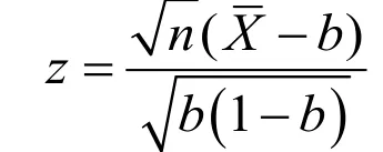
Without loss of generality, we assume d>b. For power analysis, we must also specify a known value d for p a priori, in addition to the value b under H0,in order to quantify our ability to reject H0in favor of Ha. Such explicit specification is not required for data analysis after data is observed.

Given a type I error αand a specific d in Ha,we then calculate power, or the probability that (the absolute value of) the standardized difference in (2)exceeds the threshold zα/2, i.e.,

By comparing the above with (3), we see that the only difference in (5) is the change of condition from H0to Ha. The probability in (5) is again readily evaluated to yield:

Once αis selected, power is only a function of sample size n , and b and dspecified in the null and alternative hypothesis. To determine sample size n, we must specify b and dreflect treatment effects, which are study specific and require investigators' knowledge.As power is quite sensitive to these parameters, careful consideration and justification of these quantities is critical for calculated sample size to be meaningful,reliable and informative. Thus, power analysis is not merely an algebraic and computational exercise by biostatisticians, but is an integrative process involving critical input from content researchers.

Power increases as n grows and approaches1 asn grows unbounded. Thus, by increasing sample size, we can have more power to reject the null, or ascertaining treatment effect. However, we must be mindful about selecting an appropriate power level,as arbitrarily increasing sample size not only leads to waste of precious manpower and resources, but also increases the likelihood of failed studies due to logistic constraints, and diminishing interest and return due to rapid scientific progresses and discoveries and changing technologies. Power is generally set at some reasonable level such as 0.80. Also, small treatment effect may have little clinical relevance. Thus, it is critical that we specify treatment effects that correspond to clinically meaningful differences, which again require critical input from investigators specializing in the field of study.

Given a type I error α, a pre-specified power,often denoted as 1−β, and H0and Ha, sample size is the smallest n such that the test has the given power to reject H0under Ha

Although it is generally difficult to find an analytical nformula to compute the smallest satisfying (7), such an nis readily obtained by using statistical packages.Note that power in the literature is typically denoted by 1−β, where β, known as "type II error rate", denotes the probability that the null H0is accepted when in fact it is false.

For continuous outcomes, difference µ1−µ0between µ1under Haand µ0under Hais generally expressed as an "effect size" to remove its dependence on the scale of X :

Note that for large sample size n , the z-score in(2) has approximately the standard normal distribution,which provides the basis for evaluating power using the expression in (6) when testing the hypothesis in (4).For moderate sample size, the normal approximation can still be used if np≥5and n (1 −p)≥5, where p is either p0or p1. If these conditions are not met, the z-score may deviate significantly from the normal distribution and the expression in (6) no longer provides reliable power estimates. Different methods must be used. For example, in exact inference, we use the binomial distribution of count of 1's to derive the power function.[5]Exact methods work for both small and large sample size. However, for large sample size, it takes a long time to evaluate the power function, even with modern computing power. Thus, exact methods are usually used only in cases where p or nor both are small.

3. Sample Size for Two Independent Groups

Considering testing the hypothesis,

If H0: p1−p0=0is true, the probability of rejecting H0, therefore committing a type I error a , is:

3. Sample Size for Paired Groups

In the last section, the two groups are assumed independent. This assumption is satisfied when the groups are formed by different subjects, such as male vs. female and depressed vs. healthy control subjects.In many studies, we may also be interested in changes before and after an intervention on the same individual.For example, suppose we are interested in the effect of a new antidepressant medication. We may give the drug to a group of depressed patients and measure their depression severity before and after taking the medication. Unlike groups formed by different subjects, the control (before taking the medication)and intervention (after the medication) groups are formed by the same individuals and outcomes generally become dependent between the two groups. For example, patients higher on depression severity before the mediation likely remain so after the medication.As a result, the power function for testing two independent groups discussed earlier no longer applies to such dependent "paired" groups.

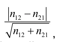
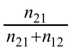
For continuous outcomes X1jand X0j, the difference Dj=X1j−X0jis also continuous. Thus, (13) becomes a hypothesis for testing whether the mean ofDjis 0 and sample size calculations can be carried out using the power function for the one group case as discussed in the previous article for power analysis for continuous outcomes. This approach, however, does not work within the current context of binary outcomes, since the difference Dj=X1j−X0jmay take on the value −1 in addition to 0 and 1 and thus no longer follows the Bernoulli distribution.

Table 1. A contingency table for joint distribution of paired binary outcomes

4. Illustrations

In this section, we illustrate power and sample size calculations for comparing two independent and two paired groups. We continue to use G*Power in our examples, as it is free and easy to use. In all cases, we set power at 80% and two-sided alpha at α=0.05.

Example 1. A San Diego-based biopharmaceutical company plans to conduct a study to test the efficacy of an experimental Ebola drug. To determine the sample size, the investigators use their pilot data and obtain the following information concerning death rates between the company's new drug and standard care:

The problem is to estimate sample size for the study to detect the above difference in death rates between the two treatment conditions.

Let p1(p0) denote the percent of death for the new drug (standard care). We can express the corresponding statistical hypothesis as follows:

To calculate sample size using the G*Power package, we enter the following information:

Statistical test > Proportions: Difference between two independent proportions

Type of power analysis > A priori: Compute required sample size – given α, power and effect size

Tails > Two

Proportion p2 > 0.22

Proportion p1 > 0.38

αerr prob > 0.05

Power (1 - β err prob) > 0.80

Allocation ratio N2/N1 > 1

By clicking on "Calculate", we obtain a sample size of 128 for each group, or a total of 256 for both groups(see Figure 1).

The G*Power also offers an exact method to calculate sample size. In this case, we enter the following information:

Test family > Exact

Statistical test > Proportions: Inequality, two independent groups (Fisher's exact test)

Tails > Two

Proportion p2 > 0.22

Proportion p1 > 0.38

αerr prob > 0.05

Power (1 - β err prob) > 0.80

Allocation ratio N2/N1 > 1

By clicking on "Calculate", we obtain a sample size of 139 for each group, or a total of 278 for both groups(see Figure 2). The estimated sample size using the exact method is slightly higher than the asymptotic method based on the standard normal distribution.Here the sample size is moderate and the discrepancy between the asymptotic and exact methods likely reflects the limited sample size. In general, if exact methods are used, we should go with sample size estimated from such methods. Fortunately, differences between asymptotic and exact methods diminish as sample size increases. Thus, such difference generally does not have any major impact on real studies.

Example 2. A research team is interested in conducting research on sexual behaviors among the Botswana Defense Force. The team has learned from other similar studies that self-reported sexual behaviors based on a daily diary is more accurate than a retrospective survey. They have estimated that about 50% would report having sex with spouse within last two weeks by daily diary, while only 20% would report such events by retrospective recall. Before conducting the survey, the research team wants to confirm such discrepancy to justify their use of a daily diary for their study.

Figure 1. Screenshot of G*Power for calculating sample size for comparing two independent proportions using the asymptotic method for Example 1

Let p1(p0) denote the percent of sex reported in a daily diary (retrospective recall). Then, the team's interest can be stated in a hypothesis as:

Since both daily diary and retrospective recall are completed by the same subject, the outcomes from the diary and retrospective recall are not independent.Thus, we use McNemar's test for comparing sexual behaviors reported by the two assessment strategies and estimate sample size using the method for paired groups.

To use the G*Power, we need to enter the odds ratio and proportion of discordant pairs under Ha. To compute these quantities, it is helpful to create the following 2x2 table indicating both the marginal probabilities p1(p0) (specified in the hypothesis)and joint probabilities (calculated from the marginal probabilities).

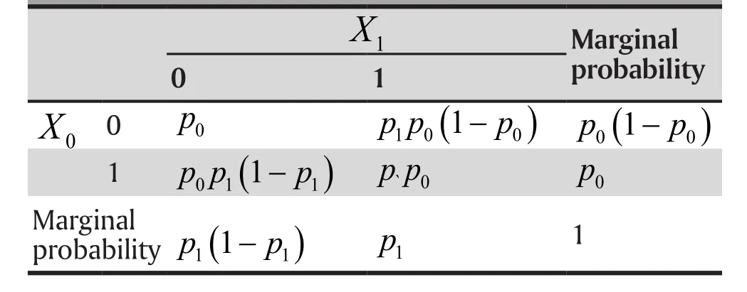
Table 2. Marginal and joint cell probabilities for the marginal and joint distribution of paired binary outcomes.

Both the odds ratio and proportion of discordant pairs are readily computed from the above table:

Proportion of discordant pairs:

We then enter these quantities, along with some other information, into the G*Power:

Figure 2. Screenshot of G*Power for calculating sample size for comparing two independent proportions using the exact method for Example 1

Test family > Exact

Statistical test > Proportions: Inequality, two dependent groups (McNemar)

Type of power analysis > A priori: Compute required sample size – given α, power and effect size

Tails > Two

Odds ratio > 2.333

αerr prob > 0.05

Power (1 - β err prob) > 0.80

Prop discordant pairs > 0.18

By clicking on "Calculate", we obtain a sample of 273 subjects to detect the hypothesized difference in reporting sexual activities between daily diary and retrospective recall (see Figure 3).

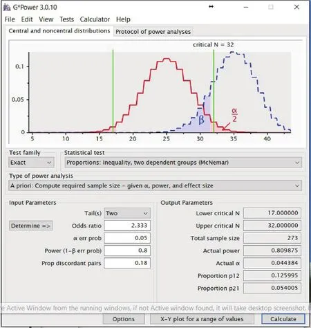
Figure 3. Screenshot of G*Power for calculating sample size for comparing two paired proportions using the asymptotic method for Example 2

4. Conclusion

Sample size estimation is an essential component of planning clinical research studies. It provides critical information for assessing feasibility of a planned study.For power analysis to be informative and useful, it requires reliable information on effect size, which can only be provided by biomedical and psychosocial investigators specializing in the field of the study. Thus,although power and sample size analysis relies on solid statistical theory, efficient computational methods and modern computing power, sample size estimates obtained from state-of-the-art methods and cuttingedge computing power are really useless without input from scientific investigators.

Funding statement

Conflicts of interest statement

The authors have no conflict of interest to declare.

Authors' contributions

Michael Zheng, Justin Tu and Xiang Lu: Manuscript outline, structure and drafting.

Michael Zheng, Jinyuan Liu and Jinyuan Liu: Technical details of statistical tests, power functions.

Jiangnan Lyn and Jinyuan Liu: Computations of sample size for illustrative examples using statistical software.

Michael Zheng, Jiangnan Lyn, Justin Tu, Jinyuan Liu,Xiang Lu: Manuscript finalizing and proofreading.

1. Chow SC, Chang M. Adaptive design methods in clinical trials.New York: Chapman & Hall / CRC; 2007

2. Heonig J M, Heisey DM. The abuse of power: the pervasive fallacy of power calculations for data analysis. Am Stat. 2001; 55(1): 19--24. doi: https://doi.org/10.1198/000313001300339897

3. Kreyszig E. Advanced Engineering Mathematics (Fourth ed.).New York: Wiley; 1979

4. Moss AJ, Zareba W, Hall WJ, Klein H, Wilber DJ, Cannom DS,et al. Prophylactic Implantation of a Defibrillator in Patients with Myocardial Infarction and Reduced Ejection Fraction. N Engl J Med. 2002; 346: 877--883. doi: https://doi.org/10.1056/NEJMoa013474

5. Tang W, He H, Tu XM. Applied Categorical and Count Data Analysis. FL: Chapman & Hall/CRC; 2012

二分类结果组间比较的样本量计算

Zhang X, Lyn J, Tu J, Liu J, Lu X

样本量、二分类结果

Summary:Sample size is a critical parameter for clinical studies. However, to many biomedical and psychosocial investigators, power and sample size analysis seems like a magic trick of statisticians. In this paper, we continue to discuss power and sample size calculations by focusing on binary outcomes. We again emphasize the importance of close interactions between investigators and biostatisticians in setting up hypotheses and carrying out power analyses.

[Shanghai Arch Psychiatry. 2017; 29(5): 316-324.

http://dx.doi.org/10.11919/j.issn.1002-0829.217132]

1Department of Statistics, University of California, Berkeley, CA, USA

2Department of Mathematics, University of California, San Diego, CA, USA

3Department of Physical Medicine and Rehabilitation, University of Virginia School of Medicine Charlottesville, VA, USA

4Department of Family Medicine and Public Health, University of California, San Diego, CA, USA

5Department of Biostatistics and Computational Biology, University of Rochester Medical Center, Rochester, NY, USA

*correspondence: Xiang LU. Mailing address: Department of Biostatistics and Computational Biology, University of Rochester Medical Center, Rochester,NY, USA; Postcode: NY 14942; E-Mail: Xiang_Lu@URMC.Rochester.edu

no external funding.

概述:样本大小是临床研究的一个重要参数.然而,把握度和样本量分析对许多生物医学和社会心理调查者来说似乎是一个统计学家的魔术.在本文中,我们继续讨论二分类结果的把握度和样本量的计算.我们再次强调了在建立假设和进行把握度分析中调查者和生物统计学家之间密切联系的重要性.

Xunan Zhang is currently completing his BS in the department of Computer Science and Statistics, University of California - Berkeley, USA. His research interest is in the field of biostatistics.