Sample Size Calculations for Comparing Groups with Continuous Outcomes

Julia Z. ZHENG , Yangyi LI , Tuo LIN , Angelica ESTRADA , Xiang LU , Changyong FENG*

•BIOSTATISTICS IN PSYCHIATRY (40)•

Sample Size Calculations for Comparing Groups with Continuous Outcomes

Julia Z. ZHENG1, Yangyi LI2, Tuo LIN3, Angelica ESTRADA4, Xiang LU5, Changyong FENG3*

sample size, continuous outcome, clinical study, power

1. Introduction

Sample size justification is required for all clinical studies. Although commercial and online statistical software have been developed to calculate sample sizes, for many biomedical and clinical researchers, the calculation of sample size seems like a magic trick of the statisticians. When their statisticians ask them for information pertaining to sample size calculations, many do not understand why statisticians ask them for such information.

Sample size, or power analysis, should be done at the design stage of a clinical study. In general, such calculations are based on statistical distributions of test statistics pertaining to study hypotheses. For adaptive designs[1], although sample size may be adjusted according to information accumulated after the study begins, the adjustment plan is pre-specified at the design stage.

Note that for some medical journals, editors often ask authors to calculate power of their completed studies and provide such information in their manuscripts. However, such post-hoc power analysis makes no statistical sense.[2]This is because although outcomes of a real study, along with their associated test statistics, are random quantities in the design stage,they all become non-random once a study is completed and have no probabilistic interpretation. Of course,the information in a completed study can be used for designs of future relevant studies.

As study outcomes are random, what is actually observed after a study is completed may be quite different from what has been proposed in the design.However, this does not mean that the study design is wrong or the study was not executed correctly. For example, suppose X is a standard normal random variable with mean 0 and standard deviation 1. The probability that X > 1.96 or X < -1.96 is 0.05. Thus,although we usually get a value of X within the range-1.96 to 1.96 when sampling X, there is still a 5% chance that X is outside of this range. Thus, when values of X are observed outside of the range, it does not mean that our assumption about the distribution of X is wrong.

In this manuscript we discuss sample size and power calculations for continuous outcomes. We give the sample size formulas for one group, two independent groups, and two paired groups. We show how preliminary information can be used to power studies.Our paper can demystify sample size justification for biomedical and clinical researchers.

2. Sample size for one group

We first consider sample size calculations for one group.Although relatively simpler, it helps illustrate basic steps for sample size calculations.

Consider a continuous outcome X and assume it has a normal distribution (often called bell-shaped distribu ti on) with meanµand varianceσ2, denoted byX∼N(µ,σ2). It is called the standard normal distribu ti on ifµ=0andσ=1. For ease of exposi ti on,we assume first thatσis a known constant.

Consider testing the hypothesis,

whereµ0is a known constant, andH0andH1are called null and alternative hypotheses, respectively.Note that as two-sided alternatives as in (1) are the most popular in clinical research, we only focus on such hypotheses in what follows unless stated otherwise.

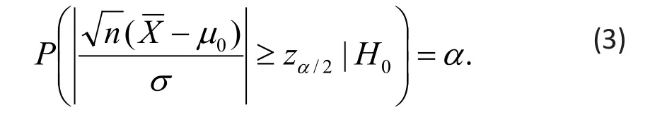
IfH0:µ=µ0is true, the probability of rejec ti ngH0,therefore committing a type I error, is readily calculated as

In clinical studies, what we are really interested in is the opposite, i.e., how we can reject the null when theH0is false. This is becauseH0usually represents no treatment effect, i.e., a straw man. Statistical power allows one to quantify the chance of rejectingH0by specifying the meanµunder the alterna ti ve, i.e.,

Without loss of generality, we assumeµ1>µ0. Note that unlike the hypothesis stated in (1), we must specify aµknown value for under the alterna ti veHaif we wish to quantify our ability to rejectH0when performing power analysis. Such explicit specification is not needed when we only test the null hypothesis after data is observed.

Given type I errorαand a specificµ1inHa, we then calculate power, or the probability that (the absolute value of) the standardized difference in (2)exceeds the thresholdzα/2, i.e.,

By comparing the above with (3), we see that the only di ff erence in (5) is the change of condi ti on fromH0toHa. The probability is again readily evaluated to yield:

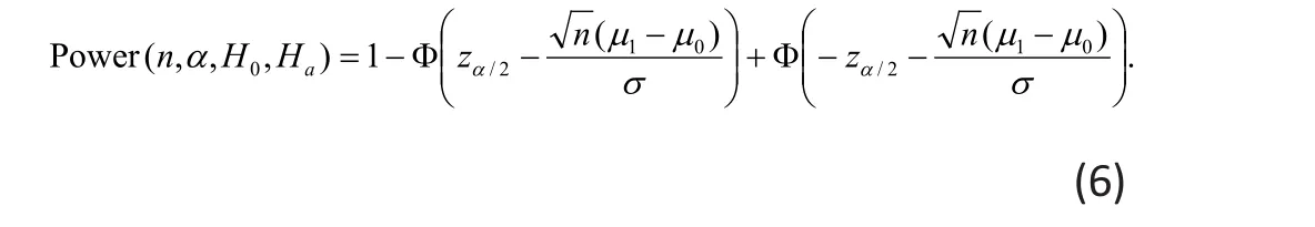
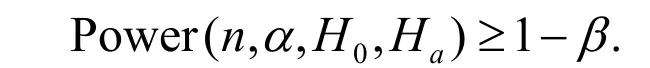
As the above shows, the power,Power(n,α,H0,Ha), isnαa func ti on of sample size , type I error and values ofµspeci fied in the nullH0and alterna ti veHa.

In most clinical research studies,µ0andµ1are posited to reflect treatment effects. Thus, onceαis selected, power is only a function of sample sizen n, which increases asngrows and approaches 1as grows unbounded. Thus, by increasing sample size, we can have more power to reject the null, or ascertaining treatment effect.

However, as increasing sample size implies higher cost for studies, power is generally set at some reasonable level such as 0.80. Also, although we can detect any small treatment effect, such statistical significance may have little clinical relevance. Thus,it is critical that we specify treatment effects that correspond to clinically meaningful differences.

Sample size justification works the opposite way.αGiven a type I error , a pre-speci fied power 1−β, andH0andHa, we want to find the smallestnsuch that the test has the given power to rejectH0underHa

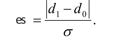
Althoughµ1−µ0measures treatment difference between the means ofXunderH0, this difference depends on the scale ofXand may change when di ff erent scales are used. For example, ifXrepresents distance,µ1−µ0will have different values if different scales are used such as mile and kilometer. Thus, effect size is used to remove such dependency:

The above is often referred to as Cohen’s d and is widely used in clinical research. In the example of distance, effect size is the same regardless of whether mile or kilometer is used.

In this case, the above arguments still apply, but the cumulative normal distribution Φwill be replaced bytthe cumulativedistribution to account for sampling variability when es ti ma ti ngσ2bys2.

3. Sample Size for Two Independent Groups

Considering testing the hypothesis,

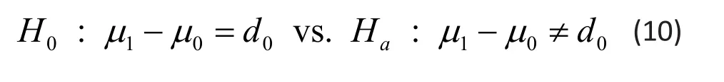
Although most clinical trials allocate equal number of subjects into groups, some studies may assign more patients to a group.[4]We assume that the number of subjects in group 0 and group 1 are n0and n1,respectively. IfH0:µ1−µ0=d0is true, the probability of rejecting H0, therefore committing type I errors, is readily calculated as:

whereαis the type I error level set a priori andzα/2is the upperα/2quan ti le of the standard normal distribution.

For power analysis, we again need to specifyµ1−µ0underHato quan ti fy the ability to reject the null when performing power analysis, i.e.,

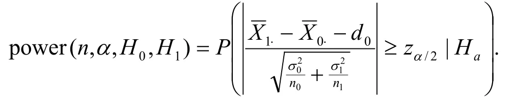
Without loss of generality, we assumed1>d0. Given a significance levelα,H0andHa, we then calculate power, or the probability that (the absolutely value of) the standardized difference in (11) exceeds the thresholdzα/2, i.e.,

As in the one-group case, we use effect size as a measure of treatment effect when calculating power. In this case, Cohen’s d is given by:

In many studies, group variances are assumed the same, in which case the effect size reduces to

Given a type I errorα, a power 1−β, andH0andHa, we can also find the smallestnsuch that the test has the given power to reject the nullH0underHa, i.e.,

4. Sample Size for Paired Groups

In the last section, data from the two groups are assumed independent. When groups are formed by different subjects, they are generally independent.In practice, we may be interested in changes before and after an intervention. For example, suppose we are interested in the effect of a newly developed drug on high blood pressure. We measure blood pressure of each subject before and after administering the drug and compare mean blood pressure between the two assessments. Since subjects with their blood pressure above the mean before the intervention are likely to stay above the mean blood pressure after the intervention, the two measures of blood pressure are not independent. As a result, the two independent group t-test does not apply to this paired group, or prepost study, setting.

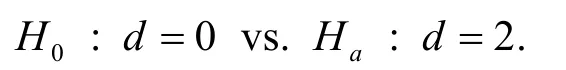
Let (Xj0j,X1j)denote the two paired outcomes from theth pair. For each pair, treatment difference isDj=X1j−X0j. If the differenceDjhas a meand=0, then there is no treatment effect. In general, we are interested in testing the hypothesis

In the two independent group case,X0jandX1kare assumed to have their own means and the hypothesis(12) involves both group means. In the current pairedgroup case, it is not necessary to identify the means ofX0jandX1j, since only the mean of differenceDjis of interest in the hypothesis (12). By comparing (4) and(13), it is readily seen that the sample size and power calculation is simply a special case of the one-group case withH0:µ=0.

5. Illustrations

In this section, we illustrate power and sample size calculations for the one group, two independent and two paired groups discussed using G*Power, a free program for power analysis, and R, a free package for statistical analysis, which also includes functions for power and sample size calculations for our current as well as more complex study settings.

The statistical hypotheses is

We set α=0.05. Although the alternative shows an increased weight, we compute power under a two-sided test. To compute power, we first convert the parameters into effect size:

When using the G*Power package, choose the following options (see Figure 1):

Test family > t tests

Statistical test > Means: Difference from constant(one sample case)

Type of power analysis > A priori: Compute required sample size

Tails > Two

Effect size d > 0.5

αerr prob > 0.05

Power (1 - β err prob) 0.80

We obtain n=34 under Total sample size in the G*Power screen.

In R, we may use the pwr package to compute power. For t-tests, use the function:

pwr.t.test(n = , d = , sig.level = , power = , type =c(“two.sample”, “one.sample”, “paired”))

where n is the sample size, d is the effect size, and type indicates a two-sample t-test, one-sample t-test or paired t-test. For each function, entering any three of the four quantities (effect size, sample size, significance level, power) and the fourth is calculated.

Using the function pwr.t.test (d = 0.5 , sig.level = 0.05, power = 0.8 , type = “one.sample”), we obtainn=33 after rounding to the nearest integer.

The statistical hypothesis is

Again, we set α=0.05 and compute power for a twosided test. Under the assumptions, the effect size is

We also assume a common group size so thatn0=n1. In G*Power package, choose the following op ti ons (see Figure 2):

Test family > t tests

Statistical test > Means: Difference between two independent means (two groups)

Type of power analysis > A priori: Compute required sample size

Tails > Two

Effect size d > 0.4

αerr prob > 0.05

Power (1 - β err prob) 0.80 Allocation ratio N2/N1 > 1

From G*Power, we obtainn0=n1=100for each group or the total sample sizen0+n1=200.

Using the function pwr.t.test (d = 0.4 , sig.level = 0.05, power = 0.8 , type = “two.sample”) in R and rounding to the nearest integer, we obtainn0=n1=99.

Figure 1. Screen shot from G*Power for Example 1

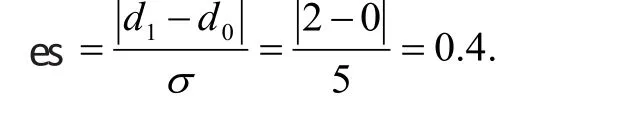
Example 3. A weight loss study using food diary wants to find a difference between pre- and postinterven ti on mean weight loss ofd=2kg. The standard devia ti on of the di ff erencedis assumedσd=5kg.

The statistical hypotheses is

We set α=0.05 and compute power for a two-sided test. The effect size is

By viewing the paired-group setting as a special case of the one-group setting, we readily obtain sample size using the following options in G*Power (see Figure 3):

Test family > t tests

Statistical test > Means: Difference from constant(one sample case)

Type of power analysis > A priori: Compute required sample size

Tails > Two

Effect size d > 0.4

αerr prob > 0.05

Power (1 - β err prob) 0.80

From G*Power, we obtain n=52.

Using the function pwr.t.test (d = 0.4 , sig.level = 0.05, power = 0.8 , type = “paired”) in R, we obtain n=51 after rounding to the nearest integer.

6. Conclusion

Sample size justification is an important consideration and a necessary component for clinical research studies.It provides critical information for assessing feasibility and clinical implications of such studies. Although power and sample size analysis relies on solid statistical theory and requires advanced computing methods,scientific investigators also play a critical role in this endeavor by providing relevant data. Without reliable input parameters, not only may power and sample size analysis be less informative, but more important potentially yield misleading information for study planning and execution.

Figure 2. Screen shot from G*Power for Example 2

Funding statement

Conflicts of interest statement

The authors have no conflict of interest to declare.

Authors’ contributions

Julia Zhang, Yingyi Li, Tuo Li and Changyong Feng:Theoretical derivation and manuscript drafting.

Angelica Estrada, Xiang Lu and Changyong Feng:Computations of power and manuscript editing.

1. Chow SC, Chang M. Adaptive design methods in clinical trials. New York: Chapman & Hall / CRC; 2007

2. Heonig JM, Heisey DM. The abuse of power: the pervasive fallacy of power calculations for data analysis.Am Stat. 2001; 55(1): 19-24. doi: http://dx.doi.org/10.1198/000313001300339897

3. Kreyszig E. Advanced Engineering Mathematics (Fourth ed.).New York: Wiley; 1979

4. Moss AJ, Zareba W, Hall WJ, Klein H, Wilber DJ, Cannom DS,et al. Prophylactic implantation of a defibrillator in patients with myocardial infarction and reduced ejection fraction.N Engl J Med. 2002; 346: 877--883. doi: http://dx.doi.org/10.1056/NEJMoa013474

比较两组连续性结果的样本计算

Zheng JZ, Li Y, Lin T, Estrada A, Lu X, Feng C

概述：所有的临床研究都需要对样本量进行辨证。然而，对于众多生物医学和临床研究人员来说，把握度和样本量看起来就像一个统计学家的魔术。在本文中，我们讨论了把握度和样本量的计算，并说明生物医学和临床研究人员在该分析的可行性和意义中具有重要作用。因此，把握度分析的确是一个互动的过程，并且科学研究人员和统计人员在研究团队中是平等合作的伙伴。

样本量、连续性结果、临床研究、把握度

Figure 3. Screen shot from G*Power for Example 3

Summary: Sample size justification is required for all clinical studies. However, to many biomedical and clinical researchers, power and sample size analysis seems like a magic trick of statisticians. In this note,we discuss power and sample size calculations and show that biomedical and clinical investigators play a significant role in making such analyses possible and meaningful. Thus, power analysis is really an interactive process and scientific researchers and statisticians are equal partners in the research enterprise.

[Shanghai Arch Psychiatry. 2017; 29(4): 250-256.

http://dx.doi.org/10.11919/j.issn.1002-0829.217101]

1Department of Immunology and Microbiology, McGill University, Montreal, Canada

2Department of Mathematics, State University of New York in Stony Brook, Stony Brook, NY, USA

3Department of Mathematics, University of California in San Diego, San Diego, CA, USA

4Department of Physics, University of California in San Diego, San Diego, CA, USA

5Department of Biostatistics and Computational Biology, University of Rochester, Rochester, NY, USA

*correspondence: Changyong Feng. Mailing address: Department of Biostatistics and Computational Biology, University of Rochester, Rochester, NY 14642,USA. E-Mail: Changyong_Feng@URMC.Rochester.edu

no external funding.

Julia Zheng is currently completing her BS in Immunology and Microbiology at McGill University,Montreal, Canada. She is preparing to expand her interest in maths and computer science by pursuing a Bachelor’s in Computer Science at University of Windsor, Windsor, Canada. In the future, Julia hopes to engage in a Master or PhD in Biostatistics to pursue her research interests in the fields of life sciences, computing biology, and biostatistics.